Advances in Food Technology and Nutritional Sciences

Open journal

ISSN 2377-8350

Translating Data into Discovery: Analysis of 10 Years of CDC Data of Mortality Indicates Level of Attainment of Education as a Suicide Risk Factor in USA

Gilberto Diaz, Jacob Jones, Toni Brandt, Todd Gary and Ashwini Yenamandra

Received: January 11th, 2017; Accepted: February 16th, 2017; Published: February 16th, 2017

INTRODUCTION

Developing a zero-suicide culture in a healthcare system requires the application of data driven quality improvement to identify at risk patients and measure the outcomes of preventative care to eliminate suicide as a leading cause of death in the United States. Variability in patient behavior and health care provider observations and assessments lead to subjective measures of risk factors that create data quality issues impeding the ability of healthcare systems to standardize data collection to discern meaningful information from their data.

Problem Space 

• Suicide rates continue to rise in the United States
• Suicide ideation, attempt and mortality data quality reporting integrity
• Systematic adoption of suicide risk identification and prevention protocols
• Significant monetary impact to the United States

Rising Suicide Rates 

A data driven quality improvement to identify suicidal patients and implement preventative measures has been difficult by healthcare systems. Despite the efforts of the organizations to prevent suicide, the CDC data revealed 400,349 suicide related deaths, marking a 2.8% increase per year 2003 to 2013. Amongst the reported deaths, the epidemic affects white, middle-aged males with a 12th grade education attainment level the most out of the United States population. The subset of 17 variables from the CDC revealed the following notable information (Table 1).


Table 1:  Data Subset Summary Statistics.
Suicide deaths by gender
Male

315,175

Female

85,174

Suicide deaths by race (Top four of fifteen)
White Non-Hispanic

334,184

White Hispanic

27,334

Black

23,355

American Indian

4,720

Suicide deaths by education attainment level
High School Diploma

70,195

Some college, Bachelor and Advanced Degrees

57,198


Data Quality Reporting

Attainment of beneficial and accurate suicide ideation, attempt and mortality data is a barrier to healthcare systems to truly capture the scope of the suicide epidemic in the United States. Western Michigan University (2016) established a Suicide Prevention Program that outlines some of the barriers impacting research, identification and prevention efforts. These are2:

• Provide an incomplete picture of the problem of suicidal behavior: Most suicide attempts do not result in death and are not included in mortality data
• Despite better reporting than morbidity data, not all suicides are reported: Sometimes there is not enough information to determine intent. Without conclusive evidence, potential suicides may be recorded as unintentional or undetermined on death certificates
• Less completely reported: While psychologically serious, many suicide attempts are not medically serious enough to require medical attention and do not get reported/coded
• Captures a biased view of the suicide injury problem: Hospital datasets are more accessible for public health surveillance than data from private physicians, clinics, and health maintenance organizations. However, hospital data may under- or over-represent certain sub-groups
• More difficult to accurately collect data about the way people feel or think versus how they behave
• Subject to reporting biases. For example, high school students are asked on the youth risk behavior survey if they ever seriously considered suicide. This question is subject to recall bias (not all people will remember), social desirability bias (not all will want to admit suicidal feelings, even on an anonymous survey), and to definition issues. After all, what is meant by “seriously” considered suicide?

Identification and Prevention Protocols 

Suicide is a sensitive subject for many people suffering from a mental illness, a traumatic event, friends and families with suicidal loved ones, school systems and even healthcare providers. The solution to treating the United States suicide epidemic will not be a simple solution. However, research suggests that a zero-suicide culture adopted from a systematic approach can reduce and even eliminate suicide related deaths, as proven with Henry Ford Health System’s award winning Depression Care Program and Centerstone’s Crisis Care Services program.3 Positive results have been identified in these two healthcare facilities; however, the United States healthcare system is extremely large, highly regulated and financially burdened. The implementation of programs like the EDC’s Zero Suicide initiative would require a leadership-driven culture change with how suicide prevention training is conducted within healthcare systems.4 Non-healthcare organizations and systems may not be able to take the same approach; however, as the United States begins to act to remediate the closeted conversation of mental illness and suicide, additional systematic approaches can be developed for a greater national impact.

Monetary Impact 

Suicide related deaths take an enormous toll on society in the United States. Aside from the emotional ramifications, the CDC reported in 2010 that suicide related death cost $44.6 billion USD for ages 10 and older. The seemingly large figure is calculated upon the combination of medical and work lost cost. Each suicide related death is reported to impact society at a rate of $1,164,499 USD. The application of this figure to the 400,349 suicidal related deaths from 2003 to 2013 amounts to a cumulative cost of $466,206,010,151.

MOTIVATION

The CDC recognizes suicide is one of leading cause of death worldwide, and the United States is not an exception, accounting for 42,773 deaths in just 2013. As of 2015, suicide was the 10th highest causes of death. For years, healthcare professionals have been fighting relentlessly regarding this issue. According to Dinah Miller,5 of Psychology today suicide rates are increasing every year. In Simon’s6 article Suicide risk assessment: Is clinical experience enough? He states, “Accurate and defensible risk assessment requires a clinician to integrate a clinical judgment with the latest evidence-based practice, although accurate prediction of low base rate events, such as suicide, is inherently difficult and prone to false positives.”

According to contributors to the Assessment of Suicide Risk,7 effective suicide risk assessment, “…should distinguish between acute and chronic risk. Acute risk might be raised because of recent changes in the person’s circumstances or mental state, while chronic risk is determined by a diagnosis of a mental illness, and social and demographic factors. Suicide risk assessments are currently conducted with the following assessments:

• The Scale for Suicide Ideation (SSI)
• The Modified Scale for Suicide Ideation (MSSI)
• The Suicide Intent Scale (SIS)
• The Suicidal Affect Behavior Cognition Scale (SABCS)
• The Suicide Behaviors Questionnaire (SBQ)
• The Life Orientation Inventory (LOI)
• The Reasons for Living Inventory (RFL)
• The Nurses Global Assessment of Suicide Risk (NGASR)

Bryan and Rudd8 in Advances in the assessment of suicide risk noted that, “There are risks and disadvantages to both overestimation and under-estimation of suicide risk. Over-sensitivity to risk can have undesirable consequences, including inappropriate deprivation of patients’ rights and squandering of scarce clinical resources. On the other hand, underestimating sociality because of a dismissive attitude or lack of clinical skill jeopardizes patient safety and risks clinician liability.”

As suicide rates continue to rise, there is reason to believe the assessments that are currently in use are not comprehensively capturing the motivations and severity of being able to properly classify the suicide risk level of patients.

The purpose of this paper is to explore social and demographic factors that are currently not being utilized in assessments that could help identify the risk of suicide in people. By uncovering these indicators, we speculate insights can be gained to aid in the improvement of suicide risk assessments being utilized by healthcare professionals to positively impact the efficacy of the efforts to decrease suicide rates in the United States. If the correlation is discovered between suicide and previously ignored risk factors, actionable programs could be developed and targeted for high risk groups. These programs could be designed to help patients seeking clinical care and, as well as those at high-risk who are not actively seeking clinical help.9

Related Work 

While the CDC has gathered an extraordinarily large data set on suicides in the United States, the variables have not revealed clear motivators as to why suicides rates continue to rise. Per Miller,5 The CDC reports revealed the following:

The news from the Centers for Disease Control shows a striking increase in suicide rates. Among those ages 35 to 64 years old (the baby boomers), there is a 28% increase in suicide rates from 1999 to 2010. It holds for males (up 27%), females (up 31%), and across different regions of the country. The peaks were seen in men in their 50’s and women in their early 60’s. The gender difference continues to show that men die of suicide at three times the rate of women, and suicide is now the 4th cause of death for that age group. More people die of suicide than car accidents. The rise is most striking in non-hispanic whites and native american alaskan indians, groups that have always had the highest rates. The suicide rate is now 17 per 100,000, up from 13 per 100,000. And while we worry more about homicide, suicide rates are twice the homicide rates. Marriage is protective, as is a college education, and in fact the suicide rate in college-educated women went down.”10,11,12

Further, according to Milner et al13 in a study published in the British Journal of Psychology, not all variables are known that are strong indicators of suicide.

This study confirms that certain occupational groups are at elevated risk of suicide compared with the general employed population, or compared with other occupational groups. At greatest risk were laborers, cleaners and elementary occupations (ISCO major category 9), followed by machine operators and ship’s deck crew (ISCO major group 8). The greater risk of suicide in lower skilled occupational groups may be symptomatic of wider social and economic disadvantages, including lower education, income and access to health services.”

In addition to the non-monetary impacts of suicide, according to the CDC’s,14 there are significant financial impacts to society:

• Suicide costs society over $44.6 billion a year in combined medical and work loss costs
• The average suicide costs $1,164,499

The majority of the individual suicide cost is a result of the work-loss amounting in $1,160,655 and the total amount increases once the average medical cost of $3,646 is calculated.15 The monetary impact to society was explored in Suicide and Suicidal Attempts in the United States: costs and Policy Implications. Sheppard et al calculated the cost to society in millions by component and age range in the following Tables 2 and 3.16


Table 2: Suicide Breakdown Cost.
Components Males Females Total %
Medical cost
Suicides $121 $26 $146 0.3
Nonfatal suicide attempts $1,149 $388 $1,537 2.6
Total (all self-inflicted injuries) $1,270 $413 $1,684 2.9
Indirect economic cost
Suicides $43,589 $9,458 $53,047 90.8
Nonfatal suicide sttempts $3,196 $518 $3,714 6.4
Total (all self-inflicted injuries) $46,785 $9,976 $56,761 97.1
Total economic cost
Suicides $43,710 $9,483 $53,193 91.0
Nonfatal suicide attempts $4,346 $906 $5,251 9.0
Total (all self-inflicted injuries) $48,056 $10,392 $58,445 100
Source: Author’s calculation.
ªItems may not sum to totals due to rounding.


Table 3: Analysis of CDC 2013 Death Data where Education Level was Made Available
Analysis of CDC 2013 Death Data


The analysis of the CDC suicide data performed by Brandt et al1 made a case that a sample data set which only uses records where the education level of the deceased is known can be used to identify trends. The data matched national statistics around sex, marital status (Table 3) and location leading to a conclusion that these records would also reflect the education levels of the larger population.

Outline of Paper 

This paper is organized as follows. Section 1 is the introduction of the paper, containing the problem space, motivation and related work. Section 2 describes the materials and data preparation involved in analyzing and drawing meaningful conclusions. Section 3 is a discussion of the results of the various data science techniques. Section 4 discusses potential challenges. Section 5 presents the possible future work for this project. Section 6 offers a conclusion based on the results. Section 7 lists the references used in the research paper. Finally, section 8 contains tables, code, and charts of interest.

MATERIALS AND METHODS 

Data Collection 

The data was collected from The Centers for Disease Control and Prevention (CDC), http://www.cdc.gov/nchs/data_access/vitalstatsonline.htm#Mortality_Multiple. The files contain all the death records of all known deceased individuals from 2003-2013 across the United States. The data is gathered through the CDC’s National Vital Statistics Systems, with the exception of the ICD10 Codes that are sourced from the World Health Organization (WHO).17 The data files report on the 75 applicable variables for each record in respect to the deceased individual’s known demographic data, reported death indicators and ICD10 Codes.

Statistical Data Analysis 

• Step 1: The 2003-2013 death data file was downloaded in a DUSMCPUB format

• Step 2: The file required to be parsed and converted into a CSV format to be imported into RStudio. To accomplish this task, a modified python script (Appendix B) available on Git Hub, was utilized to parse the DUSMCPUB data into a CSV file.

• Step 3: After parsing file and converting into a CSV file, the data was imported into RStudio.

• Step 4: As suicide risk could be correlated to objective demographic variables, a subset of 18 variables from the original 75 variables were identified to create a subset for statistical analysis of unknown variables to suicide risk. The variables identified as potentially significant are listed in Appendix A.

• Step 5: To aid in correlation analysis and, ultimately, a linear regression model of the most significantly correlated variables, variables were assigned factor levels, except for age, as described in the Rscript in Appendix B.

• Step 6: The original data contained all causes of death in the manner of death variable; however, the research is focused only on variables correlated with the suicide value. As described, in the Rscript in Appendix A subset of data was created to contain only suicide related death.

• Step 7: According to aforementioned studies, the Education variable was likely to be highly significant to suicide risk. As described in the Rscript in Appendix C, the records without Education data were removed to clear the data set.

• Step 8: After removing the records without a reported Education level and NA’s, the subset of data contained 158,970 records.

• Step 9: A combination of RStudio and a Tableau were used to visualize the data for analysis.

RESULTS 

Description of Data Set Found and Created for Analysis 

As can be seen in the Table 4 below, the original death data file contained 27,224,858 rows and 75 variables (i.e., columns). This data was reduced to contain only death labeled as suicided, bringing the record count to 400,349. Some of these rows of data were missing education levels; these records were removed, leaving a sample size of 158,970 and 17 variables that represent demographic data that could be valuable to the research.


Table 4: Observation and Variable Counts.

Name

Observations

Variables

Original death data set

27,224,858

75

Original by suicide

400,349

18

Suicide by education

158,970

18


Potential Data Science Approach 

Potential data science approaches being explored are clustering, regression and hypothesis testing to identify any significance the 18 selected variables will have to predict the probability a subject would commit suicide. Cluster analysis or clustering is the task of grouping a set of objects in such a way that objects in the same group (called a cluster) are more similar (in some sense or another) to each other than to those in other groups (clusters). It is the main task of exploratory data mining, and a common technique for statistical data analysis, used in many fields, including machine learning, pattern recognition, image analysis, information retrieval, bioinformatics, data compression, and computer graphics.18 Regression is defined as a technique in which a straight line is fitted to a set of data points to measure the effect of a single independent variable. The slope of the line is the measured impact of that variable.19 Hypothesis testing is the use of statistics to determine the probability that a given hypothesis is true. The usual process of hypothesis testing consists of four steps namely null hypothesis, test statistic, p value and comparison of p value to an acceptable significance value called α-value to see if the effect is statistically significant, then the null hypothesis is ruled out, and the alternative hypothesis is valid.20

The rationale for applying a data science approach to the 2003-2013 CDC death dataset is the success achieved in genome sequencing using data science. In the Center for Disease Control and Prevention blog, Khoury states, “Genome sequencing of humans and other organisms has been a leading contributor to Big Data, but other types of data are increasingly larger, more diverse, and more complex, exceeding the abilities of currently used approaches to store, manage, share, analyze, and interpret it effectively. We have all heard claims that Big Data will revolutionize everything, including health and healthcare.”21 By discovering associations and understanding patterns and trends within the data, big data analytics has the potential to improve care, save lives and lower societal impact.

Findings 

The following graphs show the findings from the analysis of the 11-year period 2003-2013 (Figure 1, 2 and 3).


Figure 1: Suicide Continues to Rise Year Over Year

Suicide Continues to Rise Year Over Year


Figure 2: This Graph Supports the Idea that Education Level could be a Key Risk Factor in Suicide Prevention.

This Graph Supports the Idea that Education


Figure 3: Suicide Ratio of Male Versus Females is 4 to 1 but the Average Age is Very Similar for both.

Suicide Ratio of Male Versus Females


Rationale for using Data Set 

The CDC’s22 defines suicide as, “Death caused by self-directed injurious behavior with intent to die as a result of the behavior.” It is believed the appropriate data to find unknown suicide risk indicators from the large number variables available and data published by the CDC. In addition to the large number of variables and records, their data is reliable. According to the CDC’s,7 their suicide data is gathered through the resources:

• National Electronic Injury Surveillance System-All Injury Program (NEISS-AIP)
• National Hospital Ambulatory Medical Care Survey
• National Inpatient Sample (NIS)
• National Violent Death Reporting System
• The National Vital Statistics System
• WISQARS
• Youth Risk Behavior Surveillance System (YRBSS)


Other Federal Data Sources 

• Drug Abuse Warning Network
• National Survey on Drug Use and Health (NSDUH)


Non-Federal Data Sources 

• Pan American Health Association, Regional Core Health Data Initiative
• The American Association of Sociology
• WHO Statistical Information System (WHOSIS)


POTENTIAL CHALLENGES

There has been significant research conducted in the rise of suicide in the United States; however, the published research has been unable to produce a solution to the rise of suicide. Within the scope of this research, the potential challenges have been identified by the research team:

• The majority of the research team is new to data science and is considered non-experts in the domain. The ability to find and use the correct data science method could prove difficult
• The data set made available only accounts for the deceased and does not include any living patients. Additional data sets may be needed for a conclusive study, which may be protected information
• Managing false positives and mis-classifying someone with a high risk or low risk of committing suicide
• If an unknown variable is identified, how would information is provided to the proper people in a timely manner to help with prevention?

FUTURE WORK 

In the course of this research, the authors met with several individuals to gather a better understanding of the current work being done in the field of suicide prevention as well as insight to where the discovery could be used as a mechanism for change. Scott Ridgeway, Executive Director of the Tennessee Suicide Prevention Network, highlighted the need for a more rigor around how the data is collected not only across counties in Tennessee but across the nation, meeting notes in Appendix D. Jennifer Lockman, Program Evaluator and PhD candidate from Centerstone Research Institute, conveyed the fact that there needs to be more analysis of the data and echoed the need for more standardization of data collection, meeting notes in Appendix E. The data presented at the Tennessee Suicide Prevention Network Advisory Council Retreat reinforced what the CDC data is showing, suicide rates are increasing, meeting notes in Appendix F. These meetings showed the need for more work in Tennessee and across the nation. The next steps include getting data specific to Tennessee suicides and comparing to what is being found on the national level. Concluding if education level is a factor that can be used in prevention and if so, help support initiatives that ensure the correct data is being collected.

Using the added data, information from experts, and the updated analysis publishing again to have the highest impact is a consideration. According to Journal Selector, the top 3 journals that would have the highest impact using the abstract of this paper are: Pediatrics, American Journal of Preventive Medicine, and American Journal of Public Health.

CONCLUSION 

Due to the increasing rise of suicide in the United States, research was initiated with a data science approach to identify previously unknown indicators that could lead to the prevention of suicide in the US. Previous research has been conducted to determine indicators of suicidal deaths; however, the research was based on subjective analysis of a suicidal subject’s likelihood to commit suicide. This research sought to focus on indicators that were objective characteristics so the risk assessments conducted on suspected suicidal patients could potentially increase the accuracy of the risk assessment study. The studies reviewed prior to forming the research question did not utilize data science approaches to reach their conclusions that lower education levels and labor intensive occupations lead to a higher suicidal risk. It is believed that a linear regression model can be formed to fit the variables identified in the Center for Disease Control’s death datasets from 2003-2013 that are the most significantly correlated with reported suicidal death. If the model proves accurate, subjects of the populations fitting the criteria of high risk characteristics could be introduced to potentially life-saving preventative actions to reduce the probability the subject’s cause of death would be suicide.

ACKNOWLEDGMENTS 

The Authors acknowledge the CDC and the WHO for the making the data available to public and for analysis, to Scott Ridgeway for taking time to meet with the authors to discuss about TN state suicide rate and Jennifer Lockman for her insights on how data is currently being collected and suggestions of where change is needed.

CONFLICT OF INTEREST

The authors have no conflicts of interest.

1. Brandt T, Diaz G, Jones J, Gary T, Yenamandra A. A data science approach to identify previously unknown indicators that could lead to the prevention of suicide in USA. Int Clin Pathol J. 2016; 2(4): 00047. doi: 10.15406/icpjl.2016.02.00047

2. Understanding Suicide Data. 2016. Web site. https://wmich.edu/suicideprevention/basics/understanding-data. Accessed January 10, 2017.

3. ScienceDaily. Depression care program eliminates suicide. 2010. Web site. https://www.sciencedaily.com/releases/2010/05/100518170032.htm. Accessed January 10, 2017.

4. Endocrine Disrupting Chemicals (EDCs). Zero Suicide. 2012. Web site. https://www.edc.org/zero-suicide. Accessed January 10, 2017.

5. Miller D. Rising Suicide Rates: Have We Simply Failed? 2016. Web site. https://www.psychologytoday.com/blog/shrink-rap-today/201305/rising-suicide-rates-have-we-simply-failed. Accessed January 10, 2017.

6. Simon RI. Suicide risk assessment: Is clinical experience enough? J Am Acad Psychiatry Law. 2006; 34(3): 276-278. Web site. http://jaapl.org/content/34/3/276.long. Accessed January 10, 2017.

7. Assessment of suicide risk. 2016. Web site. https://en.wikipedia.org/wiki/Assessment_of_suicide_risk. Accessed January 10, 2017.

8. Bryan CJ, Rudd MD. Advances in the assessment of suicide risk. J Clin Psychol. 2006; 62(2): 185-200. doi: 10.1002/jclp.20222

9. Suicide: Risk and Protective Factors. 2015. Web site. http://www.cdc.gov/ViolencePrevention/suicide/riskprotectivefactors.html. Accessed January 10, 2017.

10. Definitions: Self-directed Violence. 2015. Web site. http://www.cdc.gov/violenceprevention/suicide/definitions.html. Accessed January 10, 2017.

11. Paddock, C. “Suicide rates rising in US, CDC report.” Medical News Today. 2016. Web site. http://www.medicalnewstoday.com/articles/309507.php. Accessed January 10, 2017.

12. Suicide Among Adults Aged 35–64 Years —United States, 1999-2010. Web site. https://www.cdc.gov/mmwr/preview/mmwrhtml/mm6217a1.htm. Accessed January 10, 2017.

13. Milner A, Spittal MJ, Pirkis J, LaMontagne AD. Suicide by occupation: Systematic review and meta-analysis. Br J Psychiatry. 2013; 203(6): 409-416. doi: 10.1192/bjp.bp.113.128405

14. Suicide: Data Sources. 2016. Web site. https://www.cdc.gov/violenceprevention/suicide/datasources.html. Accessed January 10, 2017.

15. The Double Bottom Line Impact. 2009. Web site. http://workingminds.org/bottomline.html. Accessed January 10, 2017.

16. Sheppard DS, Geruwich D, Lwin AK, Reed GA, Silverman MM. Suicide and suicidal attempts in the United States: Costs and policy implications. Suicide Life Threat Behav. 2015; 46(3): 352-362. doi: 10.1111/sltb.12225

17. WHO. Suicide. 2016. Web site. http://www.who.int/mediacentre/factsheets/fs398/en/. Accessed January 10, 2017.

18. Wikipedia: Cluster Analysis. Web site. https://en.wikipedia.org/wiki/Cluster_analysis. Accessed January 10, 2017.

19. Kutner MH. Applied Linear Statistical Models. Chicago, IL, USA: Irwin; 1996; 4: 318.

20. Weisstein EW. “Hypothesis Testing.” From Math World–A Wolfram Web Resource. 2016. Web site. http://mathworld.wolfram.com/HypothesisTesting.html. Accessed January 10, 2017.

21. Khoury MJ. Public Health Approach to Big Data in the Age of Genomics: How Can we Separate Signal from Noise? 2014. Web site. http://blogs.cdc.gov/genomics/2014/10/30/public-health-approach/. Accessed January 10, 2017.

22. Suicide: Consequences. 2015. Web site. http://www.cdc.gov/violenceprevention/suicide/consequences.html. Accessed January 10, 2017.


APPENDIX


Appendix A:  Data Subset Variables.

Residence Status

Education

Month of Death Sex Age Value

Place of Death

Marital Status Day of Week Data_year injured_at_work manner_of_death activity_code
place_of_causal_injury icd10 race_recode3 race_recode5 hispanic_origin_recode


Appendix B:  Python Script.
 

“””

Lipscomb University: Data Science Project.


Authors: Gilberto Diaz | Toni Brandt | Jacob James | Ashwini Yenamandra


Data Analysis of Suicide from 2003 to 2013.

– This script will parse CDC’s death data sets and save it as .csv.

– This script was found on github and modified to correctly parse all 11

years data sets.

“””


fileObj = open(‘VS12MORT.DUSMCPUB’, ‘r’)

fileOutObj = open(‘mort_2012.csv’, ‘a’)


fileOutObj.write(‘Resident_Status, Education, Month_Of_Death, Sex, Age_Key, ‘ +

‘Age_Value, Age_Sub_Flag, Age_Recode_52, Age_Recode_27, ‘ +

‘Age_Recode_12, Infant_Age_Recode_22, Place_Of_Death, ‘ +

‘Marital_Status, DOW_of_Death, Data_Year, Injured_At_Work, ‘ +

‘Manner_Of_Death, Method_Of_Disposition, Autopsy, ‘ +

‘Activity_Code, Place_Of_Causal_Injury, ICD10, ‘ +

‘Cause_Recode_358, Cause_Recode_113, ‘ +

‘Infant_Cause_Recode_130, Cause_Recode_39, ‘ +

‘Entity_Axis_Conditions, EAC1, EAC2, EAC3, EAC4, EAC5, ‘ +

‘EAC6, EAC7, EAC8, EAC9, EAC10, EAC11, EAC12, EAC13, ‘ +

‘EAC14, EAC15, EAC16, EAC17, EAC18, EAC19, EAC20, ‘ +

‘Record_Axis_Conditions, RA1, RA2, RA3, RA4, RA5, RA6, ‘ +

‘RA7, RA8, RA9, RA10, RA11, RA12, RA13, RA14, RA15, RA16, ‘ +

‘RA17, RA18, RA19, RA20, Race, Race_Bridged, ‘ +

‘Race_Imputation, Race_Recode_3, Race_Recode_5, ‘ +

‘Hispanic_Origin, Hispanic_Origin_Recode\n’)


outStr = ‘’


for line in fileObj:

Resident_Status = line[19].strip()

Education = line[60:62].strip()

Month_Of_Death = line[63:67].strip()

Sex = line[68].strip()

Age_Key = line[69].strip()

Age_Value = line[70:73].strip()

Age_Sub_Flag = line[73].strip()

Age_Recode_52 = line[74:76].strip()

Age_Recode_27 = line[76:78].strip()

Age_Recode_12 = line[78:80].strip()

Infant_Age_Recode_22 = line[80:82].strip()

Place_Of_Death = line[82].strip()

Marital_Status = line[83].strip()

DOW_of_Death = line[84].strip()

Data_Year = line[101:105].strip()

Injured_At_Work = line[105].strip()

Manner_Of_Death = line[106].strip()

Method_Of_Disposition = line[107].strip()

Autopsy = line[108].strip()

Activity_Code = line[143].strip()

Place_Of_Causal_Injury = line[144].strip()

ICD10 = line[145:149].strip()

Cause_Recode_358 = line[149:152].strip()

Cause_Recode_113 = line[153:156].strip()

Infant_Cause_Recode_130 = line[156:159].strip()

Cause_Recode_39 = line[159:161].strip()

Entity_Axis_Conditions = line[162:164].strip()

EAC1 = line[164:171].strip()

EAC2 = line[171:178].strip()

EAC3 = line[178:185].strip()

EAC4 = line[185:192].strip()

EAC5 = line[192:199].strip()

EAC6 = line[199:206].strip()

EAC7 = line[206:213].strip()

EAC8 = line[213:220].strip()

EAC9 = line[220:227].strip()

EAC10 = line[227:234].strip()

EAC11 = line[234:241].strip()

EAC12 = line[241:248].strip()

EAC13 = line[248:255].strip()

EAC14 = line[255:262].strip()

EAC15 = line[262:269].strip()

EAC16 = line[269:276].strip()

EAC17 = line[276:283].strip()

EAC18 = line[283:290].strip()

EAC19 = line[290:297].strip()

EAC20 = line[297:304].strip()

Record_Axis_Conditions = line[340:342]

RA1 = line[343:348].strip()

RA2 = line[348:353].strip()

RA3 = line[353:358].strip()

RA4 = line[358:363].strip()

RA5 = line[363:368].strip()

RA6 = line[368:373].strip()

RA7 = line[373:378].strip()

RA8 = line[378:383].strip()

RA9 = line[383:388].strip()

RA10 = line[388:393].strip()

RA11 = line[393:398].strip()

RA12 = line[398:403].strip()

RA13 = line[403:408].strip()

RA14 = line[408:413].strip()

RA15 = line[413:418].strip()

RA16 = line[418:423].strip()

RA17 = line[423:428].strip()

RA18 = line[428:433].strip()

RA19 = line[433:438].strip()

RA20 = line[438:443].strip()

Race = line[444:446].strip()

Race_Bridged = line[446].strip()

Race_Imputation = line[447].strip()

Race_Recode_3 = line[448].strip()

Race_Recode_5 = line[449].strip()

Hispanic_Origin = line[483:486].strip()

Hispanic_Origin_Recode = line[487].strip()


outStr = (Resident_Status + ‘, ‘ + Education + ‘, ‘ + Month_Of_Death +

‘, ‘ + Sex + ‘, ‘ + Age_Key + ‘, ‘ + Age_Value + ‘, ‘ +

‘, ‘ + Age_Sub_Flag + ‘, ‘ + Age_Recode_52 + ‘, ‘ +

‘, ‘ + Age_Recode_27 + ‘, ‘ + Age_Recode_12 + ‘, ‘ +

‘, ‘ + Infant_Age_Recode_22 + ‘, ‘ + Place_Of_Death +

‘, ‘ + Marital_Status + ‘, ‘ + DOW_of_Death + ‘, ‘ + Data_Year +

‘, ‘ + Injured_At_Work + ‘, ‘ + Manner_Of_Death + ‘, ‘ +

‘, ‘ + Method_Of_Disposition + ‘, ‘ + Autopsy + ‘, ‘ +

‘, ‘ + Activity_Code + ‘, ‘ + Place_Of_Causal_Injury + ‘, ‘ +

‘, ‘ + ICD10 + ‘, ‘ + Cause_Recode_358 + ‘, ‘ +

‘, ‘ + Cause_Recode_113 + ‘, ‘ + Infant_Cause_Recode_130 + ‘, ‘ +

‘, ‘ + Cause_Recode_39 + ‘, ‘ + Entity_Axis_Conditions + ‘, ‘ +

‘, ‘ + EAC1 + ‘, ‘ + EAC2 + ‘, ‘ + EAC3 + ‘, ‘ + EAC4 + ‘, ‘ +

‘, ‘ + EAC5 + ‘, ‘ + EAC6 + ‘, ‘ + EAC7 + ‘, ‘ + EAC8 + ‘, ‘ +

‘, ‘ + EAC9 + ‘, ‘ + EAC10 + ‘, ‘ + EAC11 + ‘, ‘ + EAC12 + ‘, ‘ +

‘, ‘ + EAC13 + ‘, ‘ + EAC14 + ‘, ‘ + EAC15 + ‘, ‘ + EAC16 +

‘, ‘ + EAC17 + ‘, ‘ + EAC18 + ‘, ‘ + EAC19 + ‘, ‘ + EAC20 +

‘, ‘ + Record_Axis_Conditions + ‘, ‘ + RA1 + ‘, ‘ + RA2 + ‘, ‘ +

‘, ‘ + RA3 + ‘, ‘ + RA4 + ‘, ‘ + RA5 + ‘, ‘ + RA6 + ‘, ‘ + RA7 +

‘, ‘ + RA8 + ‘, ‘ + RA9 + ‘, ‘ + RA10 + ‘, ‘ + RA11 + ‘, ‘ +

‘, ‘ + RA12 + ‘, ‘ + RA13 + ‘, ‘ + RA14 + ‘, ‘ + RA15 + ‘, ‘ +

‘, ‘ + RA16 + ‘, ‘ + RA17 + ‘, ‘ + RA18 + ‘, ‘ + RA19 + ‘, ‘ +

‘, ‘ + RA20 + ‘, ‘ + Race + ‘, ‘ + Race_Bridged + ‘, ‘ +

‘, ‘ + Race_Imputation + ‘, ‘ + Race_Recode_3 + ‘, ‘ +

‘, ‘ + Race_Recode_5 + ‘, ‘ + Hispanic_Origin + ‘, ‘ +

‘, ‘ + Hispanic_Origin_Recode + ‘\n’)


fileOutObj.write(outStr)


print(“Parse complete.”)

fileOutObj.close()

fileObj.close()


Appendix C:  R Script from R Studio.
 

“””

title: “Suicide 2003-2013”

author: “Gilberto Diaz | Jacob Jones | Ashwini Yenamandra | Toni Brandt”

date: “July 2, 2016”

output: html_document


—-


# Data & Environment Preparation


“`{r setup, include=FALSE}

knitr::opts_chunk$set(echo = TRUE)

“`


### Set working environment


“`{r setwd}

setwd(‘~/Documents/r_projects/practicum_1/cdc_mortality_2003_2012/suicide_2013_2003/’)

“`


### Loading libraries


“`{r libraries, message = FALSE}

library(dplyr)

library(ggplot2)

library(gridExtra)

library(rmarkdown)

“`


### Loading suicide data sets by year (2003-2013).


“`{r, warning = FALSE, message = FALSE}

suicide.2003 <- read.csv(file = ‘suicide.final.2003.csv’,

header = TRUE,

stringsAsFactors = FALSE)

suicide.2003 <- tbl_df(suicide.2003)


suicide.2004 <- read.csv(file = ‘suicide.final.2004.csv’,

header = TRUE,

stringsAsFactors = FALSE)

suicide.2004 <- tbl_df(suicide.2004)


suicide.2005 <- read.csv(file = ‘suicide.final.2005.csv’,

header = TRUE,

stringsAsFactors = FALSE)

suicide.2005 <- tbl_df(suicide.2005)


suicide.2006 <- read.csv(file = ‘suicide.final.2006.csv’,

header = TRUE,

stringsAsFactors = FALSE)

suicide.2006 <- tbl_df(suicide.2006)


suicide.2007 <- read.csv(file = ‘suicide.final.2007.csv’,

header = TRUE,

stringsAsFactors = FALSE)

suicide.2007 <- tbl_df(suicide.2007)


suicide.2008 <- read.csv(file = ‘suicide.final.2008.csv’,

header = TRUE,

stringsAsFactors = FALSE)

suicide.2008 <- tbl_df(suicide.2008)


suicide.2009 <- read.csv(file = ‘suicide.final.2009.csv’,

header = TRUE,

stringsAsFactors = FALSE)

suicide.2009 <- tbl_df(suicide.2009)


suicide.2010 <- read.csv(file = ‘suicide.final.2010.csv’,

header = TRUE,

stringsAsFactors = FALSE)

suicide.2010 <- tbl_df(suicide.2010)


suicide.2011 <- read.csv(file = ‘suicide.final.2011.csv’,

header = TRUE,

stringsAsFactors = FALSE)

suicide.2011 <- tbl_df(suicide.2011)


suicide.2012 <- read.csv(file = ‘suicide.final.2012.csv’,

header = TRUE,

stringsAsFactors = FALSE)

suicide.2012 <- tbl_df(suicide.2012)


suicide.2013 <- read.csv(file = ‘suicide.final.2013.csv’,

header = TRUE,

stringsAsFactors = FALSE)

suicide.2013 <- tbl_df(suicide.2013)

“`


### Binding all suicide data sets into one dataframe.


“`{r, warning = FALSE, message = FALSE}

suicide.11.years <- rbind(suicide.2003, suicide.2004, suicide.2005, suicide.2006,

suicide.2007, suicide.2008, suicide.2009, suicide.2010,

suicide.2011, suicide.2012, suicide.2013)

“`


### Summary statistic


“`{r , message = FALSE}

ss11y <- summary(suicide.11.years)

ss11y

“`


“`{r , message = FALSE}

age.outlier = suicide.11.years %>%

filter(Age_Value == 999)


count(age.outlier)

count(age.outlier) / count(suicide.11.years) * 100

“`


|Variable|Description|

|:——-|:———-|

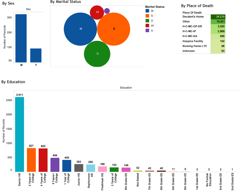
|Education|NA’s: 233733 / no education level|

|Age_Value|Max: 999 / 121 outliers; 0.03%|

|Age_Value|Mean: 46.8 / age most people suicide|

|Race_Bridged|NA’s: 398143|

|Race_Imputation|NA’s: 397188|


### Count observations by year


“`{r , message = FALSE}

suicide.by.year<- suicide.11.years %>%

group_by(Data_Year) %>%

select(Data_Year) %>%

summarise(Freq = n())


suicide.by.year


“`


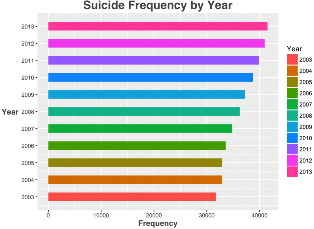
### Graphing suicide frequency by year.


“`{r, warning = FALSE, message = FALSE}

ggplot(suicide.11.years, aes(x = Data_Year, fill = factor(Data_Year))) +

geom_histogram(bins = 11, binwidth = 0.5) +

scale_x_continuous(breaks = seq(2003, 2013, 1)) +

coord_flip() +

labs(x = ‘Year’,

y = ‘Frequency’,

title = ‘Suicide Frequency by Year’,

fill = ‘Year’) +

theme(plot.title = element_text(family = ‘Helvetica’,

color = ‘#666666’,

face = ‘bold’,

size = 18)) +

theme(axis.title = element_text(family = ‘Helvetica’,

color = ‘#666666’,

face = ‘bold’,

size = 12)) +

theme(axis.title.y = element_text(angle = 360))

“`


Please notice that suicide frequency has a non stop increase for 11 years.


### Analyzing by education level.


“`{r , message = FALSE}

edu.table<- table(Education = suicide.11.years$Education, useNA = ‘always’)

edu.table

edu.table<- as.data.frame(edu.table)


edu.na.percentage<- edu.table %>%

summarise(Percentage_With_Education_Level = sum(edu.table[1:18, ‘Freq’]) / sum(edu.table[, ‘Freq’]) * 100)

edu.na.percentage

“`


Suicide for all 11 years has **400349** observations. After grouping by education level is found that **241379** observations don’t have education level reported or NA’s (empty). Therefore, the amount of **observations that do have education level is almost 40%**.


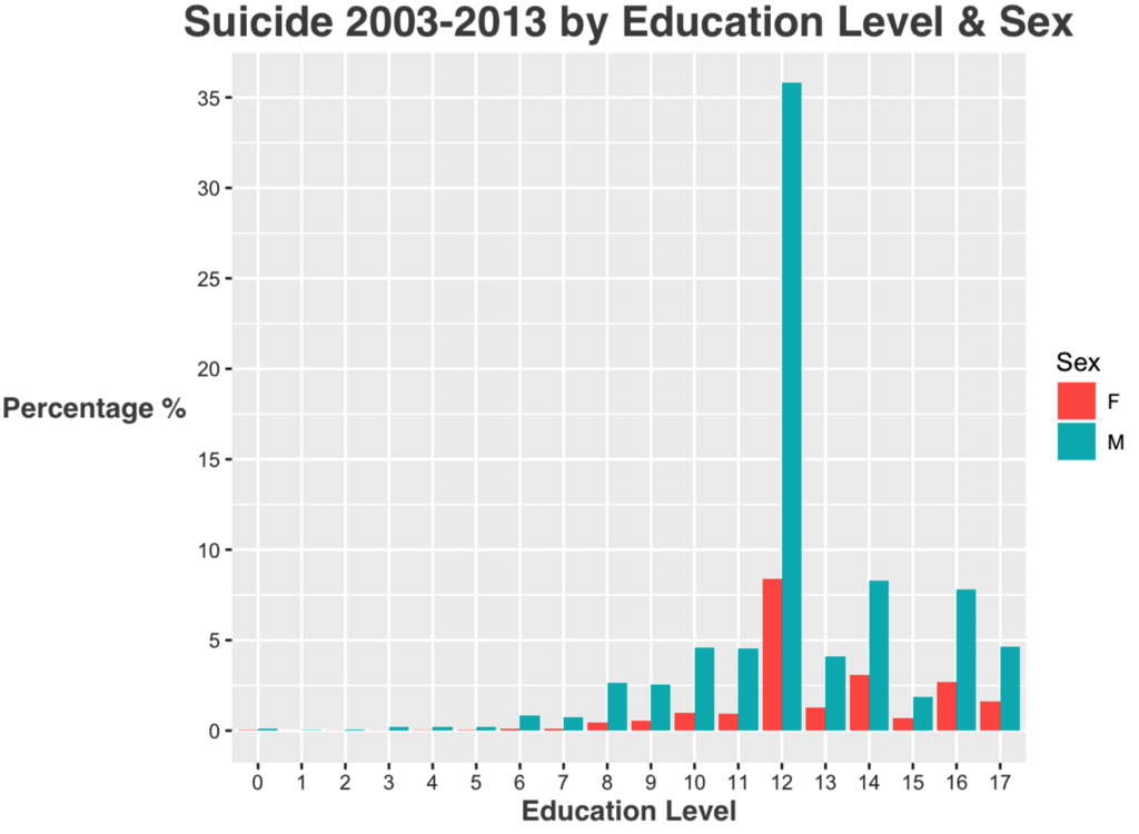
### Suicide 2003-2013 percentage group by education and sex. Observations with no education level are excluded.


“`{r, warning = FALSE, message = FALSE}

percentage.by.education.sex<- suicide.11.years %>%

filter(Age_Value<= 250, Education != ‘NA’, Education != 99) %>%

select(Resident_Status, Education, Sex) %>%

group_by(Education, Sex) %>%

summarise(Percentage = n() / length(.$Resident_Status) * 100)

percentage.by.education.sex

“`


### Percentage of people with more than a bachelor degree

“`{r, massage = FALSE}

more.bachelor<- percentage.by.education.sex %>%

filter(between(Education, 13, 17))

sum(more.bachelor$Percentage)

“`


### Graphing suicide 2003-2013 group by education & sex


“`{r, warning = FALSE, message = FALSE}

ggplot(percentage.by.education.sex, aes(x = factor(Education), y = Percentage, fill = Sex)) +

geom_bar(stat = “identity”, position = position_dodge()) +

scale_x_discrete(name = “Education Level”) +

scale_y_continuous(name = “Percentage %”,

breaks = seq(0, 40, by = 5)) +

labs(title = “Suicide 2003-2013 by Education Level & Sex”) +

theme(plot.title = element_text(family = ‘Helvetica’,

color = ‘#666666’,

face = ‘bold’,

size = 18)) +

theme(axis.title = element_text(family = ‘Helvetica’,

color = ‘#666666’,

face = ‘bold’,

size = 12)) +

theme(axis.title.y = element_text(angle = 360))

“`


|Item|Education Level Description|

|:——|:———–|

|0|No education|

|1|1st grade|

|2|2nd grade|

|3|3rd grade|

|4|4th grade|

|5|5th grade|

|6|6th grade|

|7|7th grade|

|8|8th grade|

|9|9th grade|

|10|10th grade|

|11|11th grade|

|12|12th grade|

|13|1 year of college|

|14|2 years of college|

|15|3 years of college|

|16|Bachelor degree|

|17|Bachelor +|

|99|Not state education level|


### Suicide 2003-2013 frequency by year & sex. Age_Value outlier are excluded.


“`{r, warning = FALSE, message = FALSE}

suicide.by.year.sex<- suicide.11.years %>%

filter(Age_Value<= 250) %>%

select(Resident_Status, Data_Year, Sex) %>%

group_by(Data_Year, Sex) %>%

count(Sex) %>%

rename(Count = n)


suicide.by.year.sex

“`


### Graphing suicide 2003-2013 frequency by sex.


“`{r, warning = FALSE, message = FALSE}

a1 <- ggplot(suicide.by.year.sex, aes(x = factor(Data_Year), y = Count, fill = Sex)) +

geom_bar(stat = “identity”, position = position_dodge(), width = 0.5) +

scale_x_discrete(breaks = seq(2003, 2013, 1)) +

scale_y_continuous(breaks = seq(0, 40000, by = 5000)) +

labs(x = ‘Year’,

y = ‘Frequency’,

title = ‘Suicide 2003-2013 by Year & Sex’,

fill = ‘Sex’) +

theme(plot.title = element_text(family = ‘Helvetica’,

color = ‘#666666’,

face = ‘bold’,

size = 18)) +

theme(axis.title = element_text(family = ‘Helvetica’,

color = ‘#666666’,

face = ‘bold’,

size = 12)) +

theme(axis.title.y = element_text(angle = 90))


a2 <- ggplot(suicide.by.year.sex, aes(x = Sex, y = Count, fill = Sex)) +

geom_bar(stat = “identity”, position = position_dodge(), width = 0.5) +

scale_y_continuous(breaks = seq(0, 40000, by = 10000)) +

labs(x = ‘Sex’,

y = ‘Frequency’) +

theme(plot.title = element_text(family = ‘Helvetica’,

color = ‘#666666’,

face = ‘bold’,

size = 18)) +

theme(axis.title = element_text(family = ‘Helvetica’,

color = ‘#666666’,

face = ‘bold’,

size = 12)) +

theme(axis.title.y = element_text(angle = 90)) +

facet_wrap(~ Data_Year)


grid.arrange(a1, a2, heights = 1:2)

“`


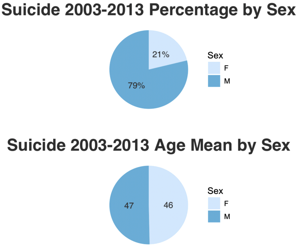
### Suicide statistic by age


“`{r, message = FALSE}

suicide.statistic<- suicide.11.years %>%

group_by(Sex) %>%

summarise(Group_Count = n(), Percentage = n() / length(.$Resident_Status),

Mean = mean(Age_Value),

Std = sd(Age_Value)) %>%

mutate(perc.pos = cumsum(Percentage) – Percentage / 2,

perc_text = paste0(round(Percentage * 100), “%”)) %>%

mutate(mean.pos = cumsum(Mean) – Mean / 2,

mean_text = round(Mean, 0))

suicide.statistic

“`


Please notice that the average age for both, male and female, are the same, 46 years old. Also notice that almost 79% of people that commit suicide are male and 21% are female.


### Graphing suicide 2003-2013 percentage & age mean by sex


“`{r , message = FALSE}

# Suicide 2003-2013 Percentage by Sex

p1 <- ggplot(suicide.statistic, aes(x = ‘’, y = Percentage, fill = Sex)) +

geom_bar(stat = “identity”, width = 1) +

geom_text(aes(y = perc.pos, label = perc_text),

size = 4,

colour = ‘#666666’,

family = ‘Helvetica’) +

coord_polar(theta = ‘y’, start = 0) +

labs(title = ‘Suicide 2003-2013 Percentage by Sex’) +

scale_fill_brewer(palette = ‘Blues’) +

theme_minimal() +

theme(axis.title.x = element_blank(),

axis.title.y = element_blank(),

axis.text.x = element_blank(),

panel.grid = element_blank(),

plot.title = element_text(family = ‘Helvetica’,

color = ‘#666666’,

face = ‘bold’,

size = 22))


# Suicide 2003-2013 Age Mean by Sex

p2 <- ggplot(suicide.statistic, aes(x = ‘’, y = Mean, fill = Sex)) +

geom_bar(stat = “identity”, width = 1) +

geom_text(aes(y = mean.pos, label = mean_text),

size = 4,

colour = ‘#666666’,

family = ‘Helvetica’) +

coord_polar(theta = ‘y’, start = 0) +

labs(title = ‘Suicide 2003-2013 Age Mean by Sex’) +

scale_fill_brewer(palette = ‘Blues’) +

theme_minimal() +

theme(axis.title.x = element_blank(),

axis.title.y = element_blank(),

axis.text.x = element_blank(),

panel.grid = element_blank(),

plot.title = element_text(family = ‘Helvetica’,

color = ‘#666666’,

face = ‘bold’,

size = 22))

grid.arrange(p1, p2)

“`


### Subset by age


“`{r, message = FALSE}

suicide.by.age<- suicide.11.years %>%

filter(Age_Value< 200) %>%

count(Age_Value)


suicide.by.age

“`


### Percentage group by Age_Value 39 to 57


“`{r , message = FALSE}

group.39.59 <- suicide.by.age %>%

filter(between(Age_Value, 39, 57))


sum(group.39.59$n) / count(suicide.11.years) * 100

“`


### Graphing suicide frequency by age


“`{r}

ggplot(suicide.by.age, aes(x = Age_Value, y = n, colour = n)) +

geom_bar(stat = “identity”, position = position_dodge()) +

scale_y_continuous(breaks = seq(0, 9000, by = 500)) +

labs(x = ‘Age’,

y = ‘Frequency’,

title = ‘Suicide 2003-2013 Frequency by Age’,

colour = ‘Frequency’) +

theme(plot.title = element_text(family = ‘Helvetica’,

color = ‘#666666’,

face = ‘bold’,

size = 18)) +

theme(axis.title = element_text(family = ‘Helvetica’,

color = ‘#666666’,

face = ‘bold’,

size = 12)) +

theme(axis.title.y = element_text(angle = 360))

“`


### Subset by ICD10:

There were many ICD10 with frequencies less than 10. I decide to create a subset that contains frequencies greater that 100.


“`{r, message = FALSE}

suicide.by.icd10 <- suicide.11.years %>%

count(ICD10) %>%

filter(n > 100) %>%

arrange(desc(n))


suicide.by.icd10

“`


|ICD10|Description|

|:—-|:———-|

|X74, X72|by discharge of firearms|

|X73|Self-harm by rifle, shotgun and larger firearm discharge|

|X70|by hanging, strangulation and suffocation|

|X60, X64|by and exposure to drugs and other biological substances|

|X61|by and exposure to drugs and other biological substances|

|X62|by and exposure to drugs and other biological substances|

|X63|by and exposure to drugs and other biological substances|

|X65, X66, X68, X69|by and exposure to other and unspecified solid or liquid substances and their vapors|

|X67|by and exposure to other gases and vapors|

|X66|by and exposure to other and unspecified solid or liquid substances and their vapors|

|X44|by and exposure to drugs and other biological substances|

|X80|by jumping from a high place|


Table is create for ICD10 with high frequency. Description for X73 was not found anywhere in the documentation files. The internet was searched for a accurate description and many websites agree that X73 description is a “Self-harm by rifle, shotgun and larger firearm discharge”. The website can be accessed [here.](http://icdlist.com/icd-10/X73.9)


### Graphing frequency of ICD10


“`{r, message = FALSE}

ggplot(suicide.by.icd10, aes(x = ICD10, y = n, fill = n)) +

geom_bar(stat = “identity”, position = position_dodge()) +

scale_y_continuous(breaks = seq(0, 150000, by = 15000)) +

labs(x = ‘ICD10’,

y = ‘Frequency’,

title = ‘Suicide 2003-2013 ICD10 Frequency’,

fill = ‘Frequency’) +

theme(plot.title = element_text(family = ‘Helvetica’,

color = ‘#666666’,

face = ‘bold’,

size = 18)) +

theme(axis.title = element_text(family = ‘Helvetica’,

color = ‘#666666’,

face = ‘bold’,

size = 12)) +

theme(axis.title.y = element_text(angle = 360),

axis.text.x = element_text(angle = 45, hjust = 1))

“`


### Calculating percentage of people that commit suicide by discharge of firearms.


“`{r}

suicide.by.icd10 %>%

filter(trimws(ICD10) %in% c(‘X74’, ‘X73’, ‘X72’)) %>%

summarise(Sum = sum(n) / nrow(suicide.11.years) * 100)

“`


Please notice that **203,146** people committed suicide by discharge of firearms.


“`{r}

percentage.by.icd10 <- suicide.by.icd10 %>%

mutate(Percentage = n / nrow(suicide.11.years) * 100)

“`


“`{r, message = FALSE}

ggplot(percentage.by.icd10, aes(x = ICD10, y = Percentage, fill = Percentage)) +

geom_bar(stat = “identity”, position = position_dodge()) +

scale_y_continuous(breaks = seq(0, 100, by = 10)) +

labs(x = ‘ICD10’,

y = ‘Percentage %’,

title = ‘Suicide 2003-2013 ICD10 Percentage’,

fill = ‘Percentage’) +

theme(plot.title = element_text(family = ‘Helvetica’,

color = ‘#666666’,

face = ‘bold’,

size = 18)) +

theme(axis.title = element_text(family = ‘Helvetica’,

color = ‘#666666’,

face = ‘bold’,

size = 12)) +

theme(axis.title.y = element_text(angle = 360),

axis.text.x = element_text(angle = 45, hjust = 1))

“`


Please notice that almost **51%** people committed suicide by discharge of firearms. That is the combination of X72, X73, and X74.


### Subset by high school diploma & committed suicide by discharge of firearms.


“`{r , message = FALSE}

# Counting all with high school diploma

hsd<- suicide.11.years %>%

filter(Education == 12) %>%

count(Education)

hsd


# Counting all with high school diploma & committed suicide by discharge of firearms.

suicide.hs.fa<- suicide.11.years %>%

filter(Education == 12, trimws(ICD10) %in% c(‘X74’, ‘X73’, ‘X72’)) %>%

count(Education)

suicide.hs.fa


# Calculating percentage of people with high school diploma & committed suicide by discharge of firearms.

suicide.hs.fa$n / hsd$n * 100

“`


Please notice that the percentage of people with an education level of high school diploma & committed suicide by discharge of firearms is **55%**, which is higher than all the people that committed suicide by discharge of firearms from 2003-2013, which is **51%**.


LATEST ARTICLES

Prevalence and Risk Factors of Subclinical Mastitis of Goats in Banadir Region, Somalia

Omar M. Salah*, Yasin H. Sh-Hassan, Moktar O. S. Mohamed, Mohamed A. Yusuf and Abas S. A. Jimale

doi.10.17140/VMOJ-9-184

Use of Black Soldier Fly (Hermetia illucens) Prepupae Reared on Organic Waste

Maggot Debridement Therapy: A Natural Solution for Wound Healing

Isayas A. Kebede*, Haben F. Gebremeskel and Gelan D. Dahesa,

doi.10.17140/VMOJ-9-183

Figure 11. Risk Map for the Introduction of Ruminant Diseases at Borders

Ovine Network in Morocco: Epizootics Spread Prevention and Identification of the At-Risk Areas for “Peste des Petits Ruminants” and “Foot and Mouth Disease”

Yassir Lezaar*, Mehdi Boumalik, Youssef Lhor, Moha El-Ayachi, Abelilah Araba and Mohammed Bouslikhane

doi.10.17140/EPOJ-8-131

The Impact of Family Dynamics on Palliative Care at the End-of-Life

Neil A. Nijhawan*, Rasha Mustafa and Aqeela Sheikh

doi.10.17140/PMHCOJ-10-154

Long-Term Follow-Up After Laparoscopic Radical Prostatectomy for Localized and Locally Advanced Prostate Cancer

Shrenik J. Shah*, Abhishek Jha, Chirag Davara, Rushi Mistry and Kapil Kachhadiya

doi.10.17140/UAOJ-7-147

Mindfulness, Sustained Attention and Post-Traumatic Stress in Tsunami Survivors

Christina Hagen*, Lars Lien, Edvard Hauff and Trond Heir

doi.10.17140/PCSOJ-2-115

Treatment and Control Methods of Bovine Mastitis: A Review

Isayas A. Kebede* and Gelan D. Dahesa

doi.10.17140/VMOJ-9-182

LATEST ARTICLES

Original Research

2024 Mar

Omar M. Salah*, Yasin H. Sh-Hassan, Moktar O. S. Mohamed, Mohamed A. Yusuf and Abas S. A. Jimale
Use of Black Soldier Fly (Hermetia illucens) Prepupae Reared on Organic Waste

review

2024 Mar

Isayas A. Kebede*, Haben F. Gebremeskel and Gelan D. Dahesa,