Study of Analysis the Sensitivity of the Computational Environment for Radiological Research Field Size Based on Two Dimensional Dose Distribution for Water Phantom Cases

Yati Hardiyanti, MSc

Department of Physics, Institut Teknologi Bandung, Jalan Ganesa 10 Bandung 40132, Indonesia; Phone. +62-8572977531; ORCID: 0000-0003-4755-6383 ; E-mail: yatihardiyanti@gmail.com

INTRODUCTION

Radiotherapy is one form of radiation therapy applications. Therefore, treatment planning in radiotherapy aims to produce a uniform dose distribution to the target volume and minimize doses beyond the target volume.^1,2 Some parameters that need to be regulated are the number of radiation beams, the radiation direction, the field size used, and the radiation’s beam weight.³ 

A technique known as intensity modulated radiation therapy (IMRT) allows a three dimensional (3D) dose distribution delivered to the patient.⁴ Photon fluency is modulated in such a way as using the multi-leaf collimator (MLC). MLC can work continuously and alternately form radiation exposure fields in either regular or irregular forms.^5,6 MLC is used to block or allow radiation to create a beam field size according to the tumor’s shape. Thus, this radiation therapy (RT) method has improved patient positioning accuracy and has led to a technique of limiting tumor movement during treatment.⁷

In IMRT optimization, it is essential to note the conformation between the level of accuracy and efficiency of the dose calculation speed. Different dosage calculation algorithms based on the IMRT technique are produced, including pencil beam (PB), Monte Carlo, and superposition/convolution. A dose calculation algorithm using the pencil beam kernel method with a semi-analytical approach has been developed.^{8,9,10,11,12,13} However, the problem faced is the efficiency of the dose calculation speed takes longer when the method is implemented in computers for clinical use. Thus, the dosage calculation algorithm using the IMRT technique was developed by Zakarian, referring to the PB dose kernel deposition pattern approach proposed by Ahnesjo et al.⁸ The algorithm is quadrant infinite beam (QIB). QIB refers to the matrix analysis that adequately represents the dose contribution of the four beam quadrants.¹⁴ The QIB algorithm is implemented in TPS software, namely computational environment for radiotherapy research (CERR), which aims to benefit research in radiation oncology treatment planning in the academic settings.¹⁵

There are many studies related to CERR used to analyze treatment planning systems and dose distribution. First, the dose distribution effect was observed in each case using five beams with the same distance. The best fluency map for IMRT procedures was identified to solve the optimization problem with the quadratic objective function. The optimal solution is obtained by the applied gradient method with a projection operation. Experiments from numerical simulations were carried out in the case of head and neck prostate. Two patient samples were taken for each case.⁷ Second, Craft developed and compared the radiation treatment optimization-planning algorithm. A collection of common optimization for radiation (CORT) datasets is provided for prostate, liver, head and neck cases the standard phantoms in the IMRT technique. The influence-dose matrix is the main form needed for optimization, in the form of a dose for each patient’s voxel from each pencil beam.⁴ In addition, Rahma has validated the QIB algorithm in the planning of nasopharyngeal cancer IMRT. In addition to the differences in the objects being studied, the dose distribution analysis was carried out by evaluating the dose volume histogram (DVH) curve and the dose colorwash.¹⁶

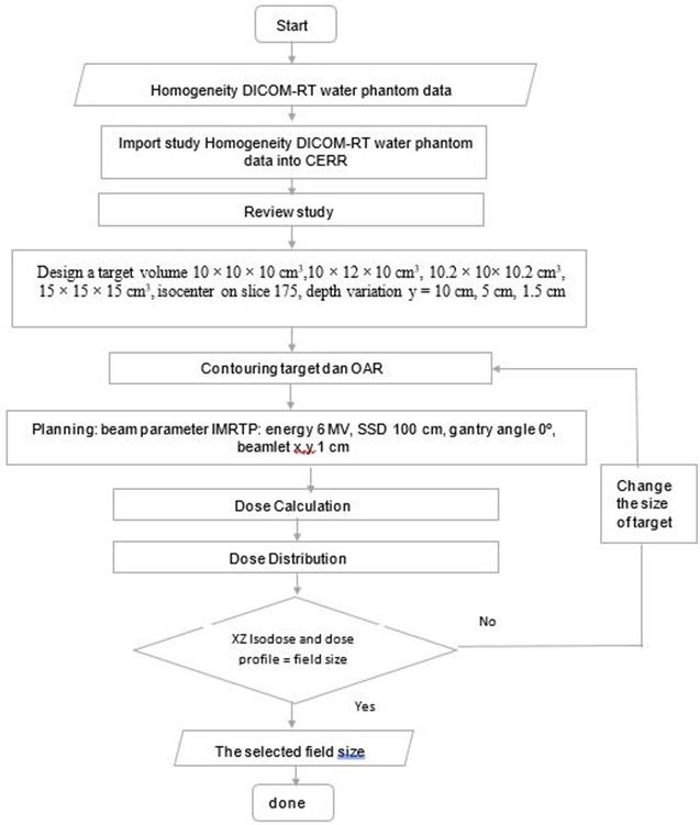
In this study, CERR was used to analyze the treatment planning system and dose distribution for water phantom cases. CERR has various analyses of dose distribution, which is displayed on 3D dose distribution, namely DVH, 2D dose distribution consisting of XY isodose curve, 1D dose distribution in the form of percentage depth dose (PDD), and dose profile analysis. The novelty described by the author is the 2D dose distribution analysis is shown in the form of an XZ isodose curve. The variations in the target volume size, depth, and position were used to analyze the dose distribution produced by CERR. This study is focused on the dose distribution analysis of the target volume shape alteration in determining the width of the field size. Thus, the purpose of this study specifically was to provide insight to be reviewed the field size sensitivity from variations in the target volume size, depth, and position, to determine the width of the field size that will contribute to the radiation beam quality control in treatment planning. In the future, this study will be used as a reference to validate the distribution of CERR dose. Thus, the accuracy of the dose calculation can be obtained (Figure 1).

Figure 1. The Flowchart of Analysis the Sensitivity of the Field Size from Variations in the Target Volume Dimensions,
Depth, and Position Based on 2D Dose Distribution

MATERIAL AND METHODS 

Material

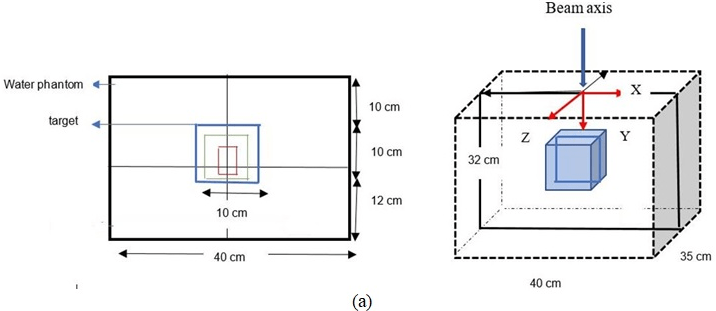
In this study, IBA dose 1 water phantom image data were used, consist of 350 slices digital imaging and communications in medicine (DICOM) format. The dimensions of the water phantom are 40×35×35 cm³.

Methods

Determination of input parameters for computational environment for radiotherapy research: First, water phantom images with DICOM format are imported into CERR and stored in planC data. Then, the water phantom image is reviewed by CERR, the target volume size modelled with dimensions 10×10×10 cm³, 10×12×10 cm³, 10.2×10×10.2 cm3, and 15×15×15 cm³, respectively. The isocenter is located on the 175^th slice. If the target volume thickness is set to 10 cm, then the target was contoured from the 125^th slice to the 225^th slice. The depth variations were set at 10 cm, 5 cm, and 1.5 cm from the surface. The design of the water phantom, and contouring target was shown in Figure 2.

Figure 2. (a) Illustration of Contouring Target Volume Design in Water Phantom (b) Beam Radiation for Variation Depth and Position

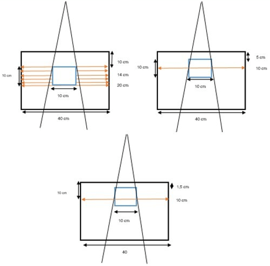
For the next step, the planning was processed based on the IMRT technique. The beam parameters used 6 MV energy, SSD 100 cm, beamlet deltax and y set at 0.1 cm for water phantom,¹⁵ also one gantry angle at the central axis of the beam 0º. The dose calculation in the central axis is essential to review.¹⁷ These parameters were chosen to observe the dose distribution along the central axis of the beam easier.

Analysis of computational environment for radiotherapy research dose distribution: The analysis of CERR dose distribution consists of the XZ isodose curve and dose profile. The XZ isodose curve indicates the field size. In Figure 2, the width of the target X-direction and the length of the target Z-direction analysis is used in determining the width and length of the field size. The field size is automatically formed from the variation target volume, which modelled 10×10×10 cm³, 10.2×10×10.2 cm³, 15×15×15 cm³ with at 10 cm, 5 cm, and 1.5 cm depths and a 10×12×10 cm³ at 10 cm depth from the surface. The XZ isodose curve is displayed as the dose distribution in each pixel. Thus, it is necessary to convert pixel units into cm units using simple mathematical equations as follows.

The calculated dose profile was obtained from the dose distribution at the 256^th pixel on the x-axis and each depth point along the y-axis. The dose distributions were then analysed 10 cm, 12 cm, 14 cm, and 16 cm, 18 cm, and 20 cm positions. The dose profile was used to compare data and justify the results of the XZ isodose curve analysis to determine the width of the field size. The dose profiles were also analysed for each depth and slice position of the target volume.

RESULTS 

Determination of Input Parameters for Computational Environment for Radiotherapy Research

From the contouring and planning results on the modelled target volume, which is based on the IMRT CERR technique, the input parameter is determined as a dose distribution for variations in 10×10 cm², 10.2×10.2 cm², and 15×15 cm² field size. The dose distribution in the target volume and organ at risk (OAR) were obtained in a 512×512×350-size dose matrix.

In this study, the results of CERR doses distribution analysis were successfully displayed in the XZ isodose curves and dose profiles, which are presented in Figure 3 and Figure 4. The XZ isodose curves for modelled targets were presented in Figures 3(a) and 3(b). The analysis of the dose was obtained from equation (III.2). The goal is to convert pixel size into cm unit so that the field size can be accurately quantized in cm unit. If the slice position is 10 cm, then the field size in X and Z axes obtained is:

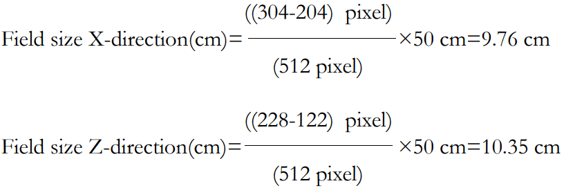
Figure 3. Dose Distribution of XZ isodose Curve for Larget Volume with Dimension 10×10×10 cm³ (a) 10×12×10 cm³ (b) depth (y=10 cm) and Position of 10 cm

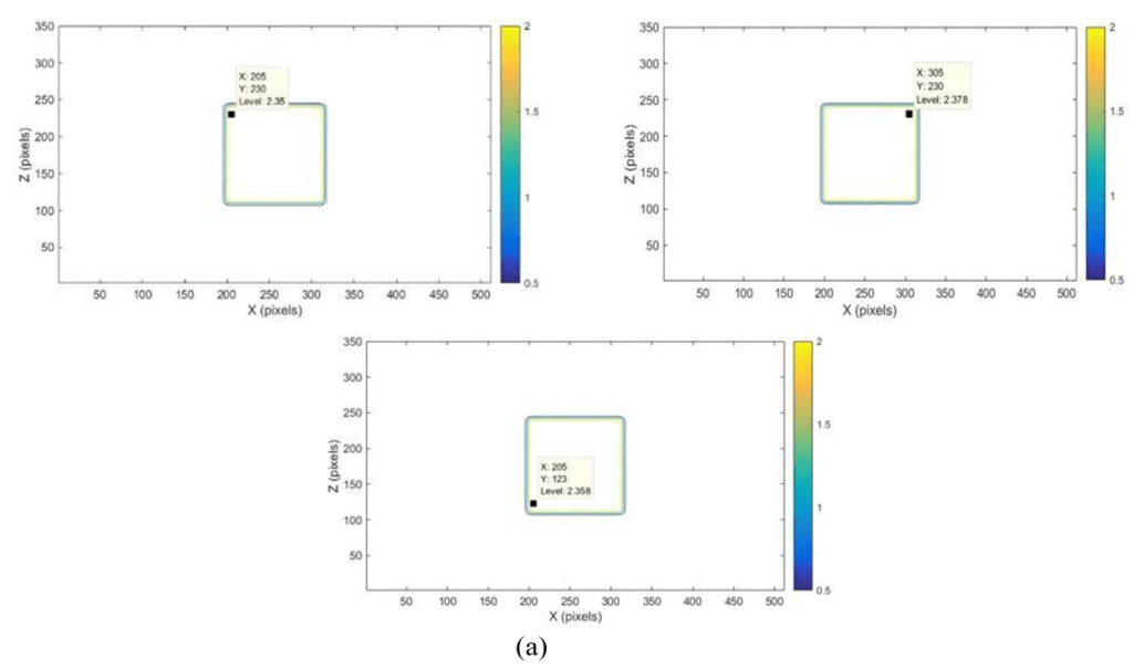
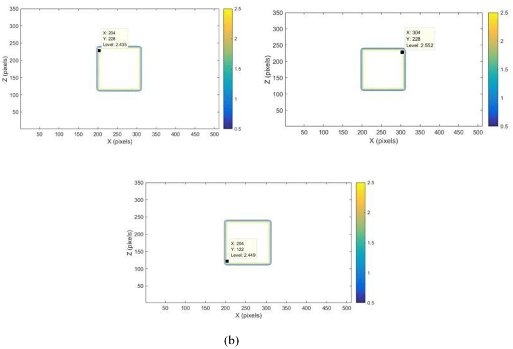
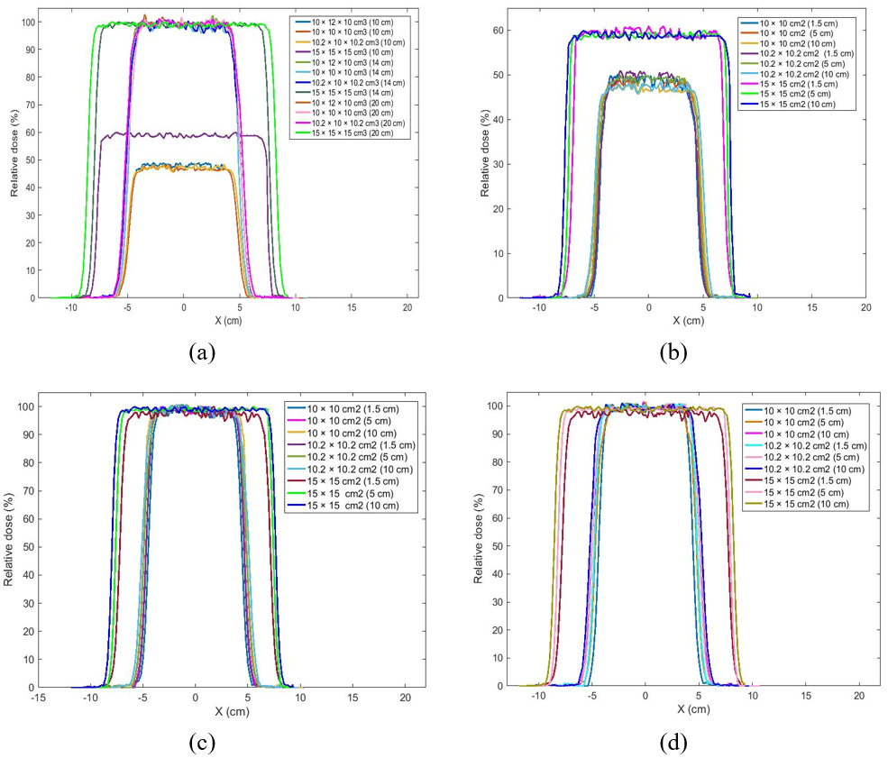
Figure 4. Comparison Beam Profile for Variation Field Size of 10×10 cm², 10.2×10.2 cm², 15×15 cm² , energy 6 MV, SSD 100 cm, Variation in the Target (a) Volume in Depth 10 cm with Variation Position of 10 cm, 14 cm, 20 cm, (b) Depth Variation of 1, 5 cm, 5 cm, 10 cm with Variation Position 10 cm, (c) 14 cm, (d) 20 cm

The analysis was applied for 12 cm, 14 cm, 16 cm, 18 cm, and 20 cm depths. The dose distribution will decrease with increasing depth from the observed position.¹⁸ The observed position’s depth was relevant to the phantom scattering, especially in the areas near the field size edge (penumbra region).¹⁷ The penumbra region usually receives doses between 80% and 20% of the beam central axis.¹⁸ The XZ isodose curve was used to determine the field size of the X-direction and Z-direction. The XZ isodose curve size was relevant to the depth of the observed position. Therefore, the results sensitivity analysis of the field size from variations in the target volume dimensions, position, and depth 10 cm were reviewed from analysis of the XZ isodose curve in Table 1. If the target volume variation and position increased, the phantom scattering also increased the field size of the X-direction and Z-direction was increased. The sensitivity of the field size of 10×10 cm² and 15×15cm² was successfully evaluated with the target volume 10×10×10 cm³, 10×12×10 cm³, dan, and 15×15×15 cm³ position variations 10 cm, 12 cm, 14 cm, 16 cm, 18 cm, 20 cm in depth 10 cm. If the target volume increased 10.2×10×10.2 cm³, the field size increase width from of 10×10 cm². While, the comparative analysis of the sensitivity for the CERR field size in the form of the XZ isodose curve was reviewed for variation in the target volume, and depth variation of 10 cm, 5 cm, and 1.5 cm depths from the water phantom surface, and slice position of 10 cm in Table 2.  If the target volume variation and depth increased, the phantom scattering also increased, the field size of the X-direction and Z-direction was increased, and the dose absorbed was decreased.¹⁹

The dose profile curve comparison results for the two modelled target volumes at a 10 cm depth in the 10 cm, 14 cm, and 20 cm slice position shown in Figure 4 (a). The dose profile is observed at the center of the beam, and then the observation point was determined in the full-width half maximum (FWHM) area. FWHM is the profile width at a 50% dose.¹⁹ The analysis result for variation in the target volume 10×10×10 cm³ and 10×12×10 cm³ showed the dose profile have similar values, at -4.9 cm to 4.9 cm for the 10 cm position, at -5 cm to 5 cm for the 14 cm position, and at -5.1 cm to 5.1 cm for the 20 cm position. If the target volume dimension 10.2×10×10.2 cm³, the width of the field size was obtained at -5.1 cm to 5.1 cm for the 10 cm position, at -5.2 cm to 5.2 cm for the 14 cm position, at -5.3 cm to 5.3 cm for the 20 cm position. If the target volume dimension 15×15×15 cm³, the field size’s width was obtained at -14.9 cm to 14.9 cm for the 10 cm position, at -15 cm to 15 cm for the 14 at -15.1 cm to 15.1 cm for the 20 cm position. Thus, the observed variation in position can influence the dose profile width. At the 10 cm and 20 cm position, the profile widths 10×10 cm² were 9.8 cm and 10.2 cm. This happened because of beam irradiation from the source to the phantom water surface.

The difference in the absorbed dose distribution was observed. The dose profile for 10×10 cm², 10.2×10.2 cm² and  15×15 cm² of 10 cm position will absorb the lower dose at around 46%, 49%, and 59% compared to 12 cm, 14 cm, 16 cm, 18 cm, and 20 composition which absorb 96% to 98% dose. The lower dose in the 10 cm position happened because it consists of planning target volume (PTV), while the other positions consist of gross target volume (GTV). Therefore, the given dose for GTV was maximized. The results of the X-ray beam profile comparison for the modelled target volume at each depth variation were shown in Figures 4 (b), 4 (c), and 4 (d). If the position was reviewed of the 10 cm in Figure 4 (b), the dose profile for 10×10 cm², 10.2×10.2 cm² field sizes had had the maximum dose of 48% at 1.5 cm depth, 47% at 5 cm depth, and 46% at 10 cm depth. The dose profile for 15×15 cm² field size was had a maximum dose of 58% at 1.5 cm depth, 57% at 5 cm depth, and 56% at 10 cm depth. If the position was reviewed of the 12 cm, 14 cm, 16 cm, 18 cm, 20 cm in Figure 4 (c) and 4 (d), the dose profile for 10×10 cm², 10.2×10.2 cm² field sizes had had the maximum dose of 99% at 1.5 cm depth, 98% at 5 cm depth, and 97% at 10 cm depth. The dose profile for 15×15 cm² field size was had the maximum dose of 100% at 1.5 cm depth, 99% at 5 cm depth, and 98% at 10 cm depth. Therefore, if the depth was increased, then the dose distribution decreased, and the profile width was increased.

DISCUSSION

The isodose curve was used to analyze the dose distribution in radiotherapy. In this study, analysis of the sensitivity of the CERR field size from variations in the target volume dimensions, depth, and position has been obtained from the XZ isodose curve analysis and dose profile. The XZ isodose curve analysis is verified with the dose profile at each observed depth and position variation. The study refers to Anam, which has developed 2D isodose curves from percentage depth dose (PDD) and dosage profiles using matrix laboratory (Matlab). The dose calculation at each point was obtained by multiplying the dose at the PDD and dose profile at 1.5 cm depth.²⁰

In its implementation, doses distribution analysis in the form of XZ isodose curves often had difficulty modelling the target volume to fit the specified field size. When this problem was found, checking the CERR input data related to the modelled target volume size for the x, y, and z directions were suggested. The next step was to adjust the modelling parameters. This is related to the process of contouring and planning beam parameters in CERR for simple geometries, such as the cube-modelled target volume and the number of gantry angles was used.

CONCLUSION

In this study, the isodose curve has been successfully displayed in the form of the XZ isodose curve to analyze the sensitivity of the CERR field size from variations in the target volume dimensions, depth, and position. The variations in the target volume analysis are used to determine the width of the field size. The XZ isodose curve is verified with the dose profile width. The calculation method was relatively valid. Variation field size of 10×10 cm², 10.2×10.2 cm², and 15×15cm² was successfully evaluated with 1.5 cm, 5 cm, 10 cm depths, and 10 cm, 12 cm, 14 cm, 16 cm, 18 cm, and 20 cm slice position variations. Thus, the quality control of the radiation beam can be obtained. In the future, this study will be used as a reference for the CERR dose distribution validation with the measurement results in the hospitals.

CONFLICTS OF INTEREST

The authors declare that they have no conflicts of interest.

1. Korhonen L. Methods for Dose Calculation and Beam Characterization in External Photon Beam Radiotherapy [dissertation]. Espoo, Finland: Helsinki University of Technology; 2009.

2. Birgani MJT, Chegeni N, Tahmasbi M, Fayazi R, Asl JF, BehrouzMA. Calculation of equivalen square fields in radiation therapy by an improved vadash correction factor for collimator exchange effects. Asian Pac J Cancer Prev. 2018; 19: 3053-3057. doi: 10.31557/APJCP.2018.19.11.3053

3. Podgorsak E. Radiation Oncology Physics: A Handbook for Teachers andStudents. Vienna, Austria: International Atomic Energi Agency; 2005.

4. Craft D, Bangert M, LongT, Papp D,Unkelbach J. Shared data for intensity modulated radiation therapy (IMRT) optimization research: The CORT dataset. Gigascience. 2014; 3(1): 37. doi: 10.1186/2047-217X-3-37

5. Clarkson JF. A note on depth doses in fields of irregular shape. J Radiol. 1941; 14: 265-268. doi: 10.1259/0007-1285-14-164-265

6. Fung AYC, Enke CA, Ayyangar KM, Thompson RB, Zhen W, Raman NV, et al. Effects of field parameters on IMRT plan quality for gynecological cancer: A case study. J Appl Clin Med Phys. 2005; 6(3): 46-62. doi: 10.1120/jacmp.v6i3.2087

7. Jahromi AF, Bozorg O, Maleki H, Mosleh-Shirazi MA. Fluence map optimization in intensity modulated radiation therapy for fuzzy target dose. Iranian Journal of Fuzzy System. 2011; 8(4): 93-105. doi: 10.22111/IJFS.2011.310

8. Ahnesjö A, Saxner M, Trepp A. A pencil beam model for photon dose calculation. Med Phys. 1992; 19(2): 263-273. doi: 10.1118/1.596856

9. Ahnesjö A, Aspradakis MM. Dose calculations for external photon beams in radiotherapy. Phys Med Biol.1999; 44: 99-155. doi: 10.1088/0031-9155/44/11/201

10. Deasy JO, BlancoAI, Clark VH. CERR: A computational environment for radiotherapy research. Med Phys. 2003; 30(5): 979-985. doi: 10.1118/1.1568978

11. Kalinin E, Deasy J. A method for fast 3-D IMRT dose calculations: The quadrant infinite beam (QIB) algorithm. Med Phys. 2003; 50(8): 1348-1349.

12. Jelen U, Sohn M, Alber M. A finite size pencil beam for IMRT dose optimization. Biol Phys Med Biol. 2005; 50(8): 1747-1766. doi: 10.1088/0031-9155/50/8/009

13. Breedveld S, Storchi P, Keijzer M, Heijmen B. Fast, multiple optimizations of quadraticdose objective functions in IMRT. Phys Med Biol. 2006; 51(14): 35-69. doi: 10.1088/0031-9155/51/14/019

14. Zakarian C, Deasy J, Kalinin E. A method for fast 3-D IMRT dose calculations: The quadrant infinite beam (QIB) algorithm. 2003; 82: 5330.

15. Apte PA. WE-D-201-02: Walk-through of CERR capabilities. Med Phys.2015; 42 (6): 3672-3672. doi: 10.1118/1.4925955

16. Rahma AY. Validation of Quadrant Infinite Beam (QIB) Algorithm for Nasopharynx Cancer Intensity Modulated Radiation Therapy (IMRT) Treatment Planning, InstitutTeknologi Bandung [master’s thesis]. Bandung, Indonesia: InstitutTeknologi Bandung; 2019.

17. Khan FM, Gibbons JP. The Physics of Radiation Therapy. Philadelphia, USA: Lippincott Williams and Wilkins; 2014: 60-172.

18. Nath R, Biggs PJ, Bova FJ, Ling CC, Purdy JA, van de Geijn J, et al. AAPM code of practice for radiotherapy accelerators report No. 47. Med Phys. 1994; 21: 1093-1121 . doi: 10.1118/1.597398

19. Karzamark CJ. Advance in linear accelerator design for radiotherapy. Med Phys. 1984; 15(4): 604-610. doi: 10.1118/1.595617

20. Anam C. Development of 2D Isodose Curve from The PDD and Dose ProfilesUsing Matlab. 2^th ISNPINSA; 2012: 48-52.