Statistical Parameters of Forensic Importance for 15 Autosomal STRs in Mestizo Population from the State of Guerrero (South Mexico)

Héctor Rangel-Villalobos, PhD

Instituto de Investigación en Genética Molecular, Universidad de Guadalajara, Centro Universitario de la Ciénega (CUCiénega-UdeG), Av. Universidad #1115, Col. Paso Blanco, CP 47810, Ocotlán, Jalisco, México; Tel. 52+ (392) 92 59400, ext. 8363;
Fax: +52 (392) 92 57112; E-mail: hrangel13@hotmail.com

INTRODUCTION

In Mexico, most of the population (>90%) is the consequence of an admixture on account of European contact principally with the Spaniards, Amerindians, and African slaves. This part of the population is commonly referred to as the Mestizos, who speak Spanish and live in both urban and rural regions throughout the country. Many studies have been conducted in Mexican-Mestizos to validate the application of autosomal short tandem repeats (STRs) for human identification purposes.^1,2 However, in Mexico, this forensic validation requires the study of different populations, given the genetic structure demonstrated among Mestizos from different regions.³ Based on the 13 STRs of the Combined DNA Index System (CODIS), it has been claimed that the European ancestry increases gradually towards the Northwestern region and diminishes towards the Central and Southeastern regions; conversely, the Amerindian ancestry displays an opposite pattern increasing towards the Central and Southeastern region, and decreasing towards the Northwestern region.^1,2 Although, several Mexican-Mestizo populations have been studied, some geographical areas have been poorly analyzed for STR markers from a forensic perspective; particularly the Southern region characterized by the presence of numerous Mexican indigenous communities, which could potentially increase the Amerindian ancestry of the neighboring southern Mestizo populations.⁴ Therefore, the two defined objectives of this study were:

1. To report the statistical parameters of forensic efficiency for 15 STRs of the Identifiler^® kit in the state of Guerrero, a representative of the southern Mestizo population;
2. To compare the collected data with the populations from the main geographical regions of Mexico.

MATERIALS AND METHODS

DNA Samples 

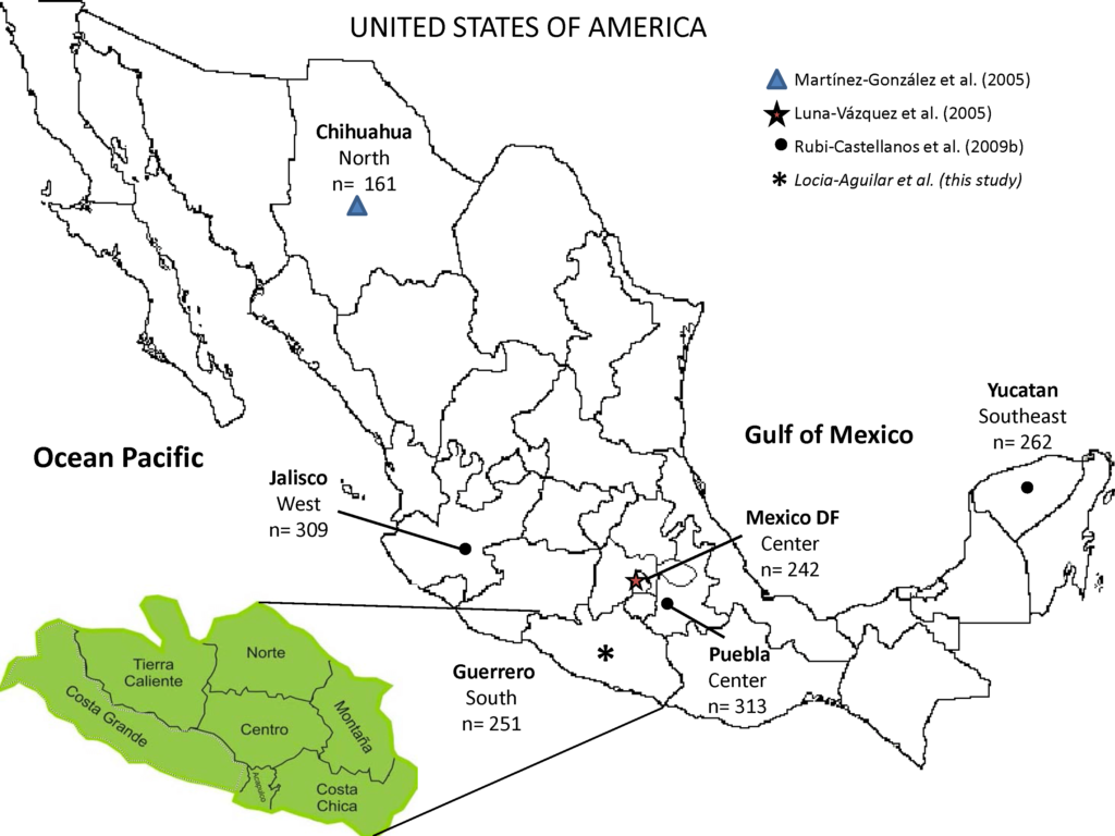
We analyzed the DNA samples of 251 unrelated Mexican-Mestizo individuals from the following regions of the southern state of Guerrero: Costa Chica (n=14), Acapulco (n=80), Centro (n=53), Montaña (n=23), Norte (n=56), and Tierra Caliente (n=25) (Figure 1). All individuals participating in the study, signed a written informed consent according to the ethical guidelines of the Helsinki Declaration.

STR Genotyping 

DNA was extracted from a dried blood specimen spotted on the FTA paper or buccal swabs using Chelex® 100 or the standard phenol-chloroform method. Genotypes for 15 STRs were obtained with the AmpFlSTR Identifiler^® kit followed by capillary electrophoresis according to the supplier´s instructions using the ABI-Prism 3130 Genetic Analyzer (Applied Biosystems, Foster City, CA, USA). Allele ladder provided in the kit and the software Genemapper^® 3.2 were used for allele calling.

Quality Control 

Positive and negative controls were used as specified in the Identifiler^® kit user’s manual. The genotype data was analyzed and verified independently by two different statistical methods.

Data Analysis 

Allele frequencies and statistical parameters of forensic efficiency were estimated with the spreadsheet PowerStats.⁵ Hardy-Weinberg equilibrium (HWE) for each and the combined loci were computed by performing the exact tests using the software Genetic Data Analysis (GDA) 1.1.⁶ Population differentiation was evaluated by performing pairwise comparisons (exact test p-value) and normalized F_ST genetic distances represented in a Multidimensional scaling (MDS) plot using the software Arlequin 3.0⁷ and Statistical Package for the Social Sciences (SPSS) version 20.0, respectively. For this purpose, four previously reported Mexican-Mestizo populations from different geographic regions were included in the interpopulational analysis: Chihuahua (North),⁸ Jalisco (West),⁹ Valley of Mexico,¹⁰ and state of Puebla (Center),⁹ and Yucatan (Southeast)⁹ (Figure 1).

Figure 1: Geographical Location, Sample Size (n) and Reference of the Mexican-Mestizo Populations Used for Interpopulation Analysis in this Study

RESULTS AND DISCUSSIONS

Allele frequencies and statistical parameters of forensic efficiency of the 15 STRs for the Identifiler^® kit have been summarized in Table 1. In addition, complete genotype STR dataset is available as electronic supplementary material in Supplementary Table 1. This information will be helpful to the Mexican forensic geneticists to evaluate paternity and forensic cases solved in the Guerrero state. According to these forensic parameters, the most informative loci were D18S51, D2S1338 and FGA; conversely, the STRs with the lowest forensic informativity were TPOX and D3S1358. The combined power of exclusion for the STR genetic system was 99.999634444%, whereas the combined power of discrimination was greater than >99.99999999%, confirming the potential of this kit for human identification purposes. Although, HWE test showed a low p-value for D21S11 (p=0.041), the application of the Bonferroni correction (p<0.0033) suggested that the genotype distribution was in agreement with the Hardy-Weinberg expectations for all the 15 STR loci in the population of Guerrero. Similarly, the exact linkage equilibrium was established between all pairs of loci (p>0.0038) (Data not shown). In brief, these results suggested that the binomial square and product rule can be confidently used in forensic caseworks to estimate DNA profiles obtained with the Identifiler^® kit in the population of Guerrero.

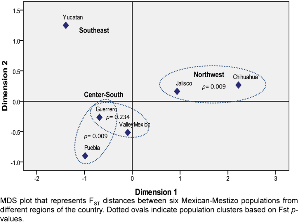
The knowledge of the genetic relationships among populations is important because it guides the work of forensic geneticists to analyze alternative STR population data during the statistical interpretation, given that most of the Mexican-Mestizo populations do not have their own STR database. Until now, this interpopulation analyses of Mestizo populations including the main geographic regions of the Mexican territory have been carried out only with the 13 CODIS-STRs.^1,2 Therefore, we represented the genetic distances among six Mexican-Mestizo populations in an multidimensional scaling (MDS) plot with the complete set of 15 STRs constituting the Identifiler kit (Figure 2). Although, recently, three Mexican Native populations from Guerrero were analyzed with these 15 STRs,¹¹ the complete genotype dataset was not available and thus, could not be included in this report. The close similarity observed between the southern state of Guerrero and the central populations is partially in agreement with the geographical parameters. However, the greater extent of similarity between the population residing in the Valley of Mexico with Guerrero (p=0.2342) than with the nearby population of Puebla (p=0.0000), disregards the idea that geography could possibly explain such genetic associations (Table 2). This observation is in agreement with the first global study conducted on Mexican-Mestizos based on CODIS-STRs that discarded the Isolation by Distance (IBD) hypothesis¹ by means of the autocorrelation indices for DNA analysis (AIDA). These contradictory results suggest that Mexican population relationships have been explained by factors such as socioeconomic conditions and educational status associated with the higher European ancestry.¹² Similarly, the IBD hypothesis has not been followed for the study of Native American populations from Mexico when geographic distances are lesser than 1500 km,¹³ which is in agreement with our results. A different quadrant of the MDS plot represents the populations of Chihuahua (North) and Jalisco (West), whereas the Yucatan population is isolated in a third different section of the plot (Figure 2). Although, this result is partially in agreement with a previous description that roughly classifies the distribution of the Mexican-Mestizo population into two principal regions (Northwest and Center-Southeast).^1,2 The observed distribution suggests that the Southeastern region is different and should be considered as independent from the Central and Southern regions.

Figure 2: MDS Plot Representing the Genetic Relationships Among Six Mexican-Mestizo Populations Based upon the Powerplex 16 System.

CONCLUSION

We estimated for the first time the forensic parameters for 15 STRs in Mestizos from Guerrero (South, Mexico). We describe the genetic structure of Mexican-Mestizos based on 15 STRs, where the Southeastern region showed differences with the Central and Southern regions. 

CONFLICTS OF INTEREST 

The authors declare that they have no conflicts of interest.

1. Rubi-Castellanos R, Martínez-Cortes G, Muñoz-Valle JF, et al. Pre-Hispanic Mesoamerican demography approximates the present-day ancestry of Mestizos throughout the territory of Mexico. Am J Phys Anthropol. 2009; 139: 284-294. doi: 10.1002/ajpa.20980

2. Salazar-Flores J, Zuñiga-Chiquete F, Martínez-Sevilla VM, et al. Admixture and genetic relationships of Mexican Mestizos regarding Latin American and Caribbean populations based on 13 CODIS-STRs. J Comparative Hum Biol HOMO. 2015; 66: 44-59. doi: 10.1016/j.jchb.2014.08.005

3. Moreno-Estrada A, Gignoux CR, Fernández-López JC, et al, The genetics of Mexico recapitulates Native American substructure and impacts biomedical traits. Science. 2014; 344: 1280-1285. doi: 10.1126/science.1251688

4. Martínez-Cortés G, Nuño-Arana I, Rubi-Castellanos R, et al. Origin and genetic differentiation of three native Mexican groups (Purépechas, Triquis, and Mayas): Contribution of CODIS-STRs to the history of human populations of mesoamerica. Ann Hum Biol. 2010; 37: 801-819. doi: 10.3109/03014461003743801

5. Tereba A. Tools for analysis of population statistics. In: Profiles in DNA: Madison, WI, USA: Promega Corp; 2001.

6. Lewis PO, Zaykin D (GDA). Genetic Data Analysis: Computer program for the analysis of allelic data version 1.0 2001. 2001. Web site. http://hydrodictyon.eeb.uconn.edu/people/plewis/software.php. Accessed May 3, 2017.

7. Excoffier L, Laval G, Scheneider S, Arlequin ver. 3.0: An integrated software package for population genetic analysis. Evol Bioinform Online. 2005; 1: 47-50. doi: 10.1177/117693430500100003

8. Martínez-González LJ, Martínez-Espín EM, Fernández-Rosado F, et al. Mexican population data on fifteen STR loci (Identifiler kit) in a Chihuahua (North Central Mexico) sample. J Forensic Sci. 2005; 50: 236-238. doi: 10.1520/JFS2004361

9. Rubi-Castellanos R, Anaya-Palafox M, Mena-Rojas E, Bautista-España D, Muñoz-Valle JF, Rangel-Villalobos H. Genetic data of 15 autosomal STRs (Identifiler kit) of Three Mexican Mestizo Population samples from the States of Yucatan (Southeast), Jalisco (West), and Puebla (Center). Forensic Sci Int Genet. 2009; 3: e71-e76. doi: 10.1016/j.fsigen.2008.07.006

10. Luna-Vázquez A, Vilchis-Dorantes G, Aguilar-Ruiz MO, et al. Population data for 15 Loci (Identifiler^® Kit) in a sample from the Valley of México. Legal Med. 2005; 7: 331-333. doi: 10.1016/j.legalmed.2005.06.002

11. López-Parra AM, Chiñas PI, Huang Q, Arroyo-Pardo E, Mesa MS. Genetic polymorphism of 15 STR loci in 3 ethnics groups of Guerrero State, Mexico. Forensic Sci Int Genet. 2016; 25: e8-e9. doi: 10.1016/j.fsigen.2016.06.018

12. Martínez-Marignac VL, Valladares A, Cameron E, et al. Admixture in Mexico City: Implications for admixture mapping of type diabetes genetic risk factors. Hum Genet. 2007; 120: 807-819. doi: 10.1007/s00439-006-0273-3

13. Rangel-Villalobos H, Martinez-Sevilla VM, Martinez-Cortes G, et al. Importance of the geographic barriers to promote gene drift and avoid (pre and post-Columbian) gene flow in Mexican Native groups: Evidence from forensic STR loci. Am J Phys Anthropol. 2016; 160(2): 298-316. doi: 10.1002/ajpa.22969