Calculation of Photons Reaction Rate Resulting at 120 kVp X-ray Tube Voltage and 1 mAs as Function to Digital Imaging and Communications in Medicine Pixel Numbers Using Monte Carlo N-Particle Transport and a Voxel Model of a 29-Year-Old Patient

Tawfik A. Shdeed, PhD

2^nd Faculty of Mechanical and Electrical Engineering, Damascus University, Syria; E-mail: ashdeedtaw@gmail.com

INTRODUCTION

Computed tomography (CT), contributes over 34% of collective dose from diagnostic X- rays examination in the world,¹ where the dose resulting from CT scanner (for whole body examination estimated at 10 mSv, while dose during conventional imaging estimated at 0.02-0.04 mSv) , therefore the  difference is very large between the two scans can be reach to 400-500 times. Because these radiations is not visible, the resulting dangers do not appear directly, but have a stochastic effects that can appear in subsequent years or generations, It was therefore necessary to adjust and monitor the radiation doses resulting from these practices and to assess the radiation risks resulting from them. Table 1 gives a comparison between the effective dose resulting from the computed tomography and each of the traditional imaging of the chest and the number of years of exposure to natural background radiation which produces the same effective dose resulting from computed tomography.¹

According to some statistics, the number of computed tomography devices in Syria exceeds 232 devices, serving more than 19 million people, where one machine serves about 86 thousand people, therefore It is necessary to assess the effects of these devices on an ongoing basis.

Matlab Program

The matrix laboratory (MATLAB) platform is optimized for solving engineering and scientific problems. The matrix-based MATLAB language is the world’s most natural way to express computational mathemati.² CT DICOM images were read using the MATLAB program in purpose to construct a three-dimensional phantom (voxels phantom), therefore, the following commands have been implemented, {DICOMINFO, DICOMREAD, IMSHOW, MIN, MAX, IMTOOL}.

Monte Carlo N–Particle Code

Monte Carlo n–particle code (MCNP) is a general-purpose MCNP that can be used for neutron, photon, electron, or coupled neutron/photon/electron transport, including the capability to calculate given values for critical systems. for photons, the code accounts for incoherent and coherent scattering, the possibility of fluorescent emission after photoelectric absorption, absorption in pair production with local emission of annihilation radiation, and bremsstrahlung.³

Purposes of the Research

To read the dicom images of brain and extract intensity values and build a three dimensional model for mcnp code input file in purpose to study the average particle flux and deposited energy of X-ray photons resulting at 120 kvp and 1 mas as function to DICOM pixel numbers in the brain tissues for a 29-year-old female patient using MCNP code and MATLAB program to read the DICOM images.

METHODS AND MATERIALS

The General CT Model

In this study was based on a ct scan of a female patient aged 29-years, using a scanner, the multislice helical ct scanner was used for all simulations. it is a third generation CT scanner quipped with solid state detectors system.

Scan time for full helical scan is 100 seconds. The operating voltage are 80, 100, 120 and 135 kVp and the tube current can vary from 30 to 300 mAs in steps of 10 mAs . Table 2 shows the specifications of the CT images and the CT scanner used for this study.

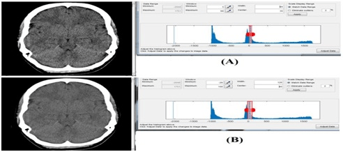
In order to get better contrast of the tissues, the following values were modified, the window’s minimum intensity value=3, the window’s maximum intensity value=68 that corresponding to window’s width=65 and window’s center=35 instead of window’s width=120 and window’s center=40. As shown in Figure 1.

Figure 1. Comparison between Two Cases of Window Intensity Values, (A) The Window’s Width=65 and
Window’s Center=35. (B) Window’s Width=120 and Window’s Center=40

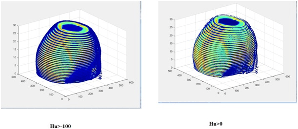
Voxel Phantom

Figure 2 shows the voxel phantom that was adopted in this study of the head region. This phantom consists of a number of voxels (512×512×100) with voxel size 0.2×0.2×1 cm³, in this case each pixel will be corresponded to one voxel, i.e. each pixel will be represented within 0.2×0.2×1 cm³. Figure 2 shows parts of this phantom plotted for the entire digital image matrix (512×512). Parts of it were displayed because of the difficulty of showing the entire phantom according to the PC used in this study. Where used In this study a computer with (core i5- CPU 2.30 GHz processor) and 1 Gb VGA. On the Figure 2, the areas appear stretch from the blue color that corresponds to the least color intensity (the lowest values for the CT number, Hu=-950, that corresponding to the air material) and upto the red color (which corresponds to the highest values for the CT number, Hu=1370, that corresponding to the Skeleton cortical bone material).

Figure 2. Parts of the Voxel Phantom Used in this Study

Materials Assign

The CT images were read using the Matlab program, after that, the images were then resized to a scale of 325×171 pixel, in accordance with the number of identical voxels in the phantom used in the study. Firstly, in the input file of MCNP code, the equivalent substances were created for air, soft brain tissue, red blood cells, spinal cord, skin, facial and skull bones, Adipose tissue, Yellow marrow, Cell nucleus, Red marrow, lymph, eye lens,.. etc. secondly, each material was given a number and a universe number (U) that corresponding to certain range of CT numbers that defined each pixel in image. The values of the chemical composition and the CT numbers (in Hounsfield) and density were taken from several references such as.^4,5,6 Table 3 shows chemical composition as percentages, density p and Hounsfield numbers for various tissue descriptions.

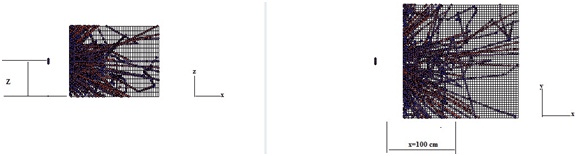
Source Modeling

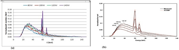
In order to determine the energy spectrum of X-ray photons emitted at certain value of tube voltage (kVp), the X-ray tube was simulated using MCNP code. the energy spectrum of the photons produced was calculated at several voltage values, as shown in Figure 3. To calculate the average particle flux and deposited energy X-ray source was simulated as point source at distance from the center of phantom equals to 100 cm on X_axis, and variable step on Z_axis Figure 4 (1).

Figure 3. The Spectrum Energy of X-ray Photons Emitted at Several Values of Tube Voltage Calculated Using the MCNP Code

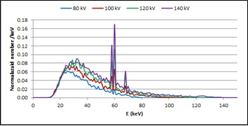
Figure 4 (1). The X-ray Point Source Modeling, X-ray Photons Distribution Using MCNP Code

Average Particle Flux in a Cell and Deposited Energy

In this study we used the “F4” (cell fluence) tally to calculate reaction rate across slice that gives a quantity in units of particle/cm² per source particle.³

The average particle flux in a cell can be written:

Where:    is the density of particles.

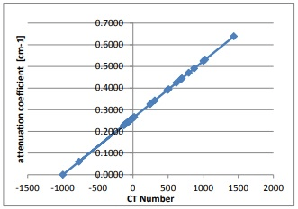
Cell heating and energy deposition tallies are track length flux tallies modified totally a reaction rate convolved with an energy-dependent heating function, The units of the heating tally are MeV/g, the heating number H(E) for photons is³:

Where: i=1 incoherent (Compton) scattering with form factors, i=2 pair production;

(E)=2m₀c²=1.022016 MeV, i=3 photoelectric absorption (E)=0 p_t (E): probability of reaction i at gamma incident energy E.

(E) average exiting gamma energy for reaction i at photon incident energy E.

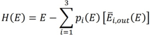
RESULTS

As have been explained previously, all calculations were done for point source at 1 mAs and 120 kVp and 4 mm slice thickness. Table  4 shows the average of de posited energy in (MeV/g/1mAs), mean free path, and mass attenuation coefficient as function to CT numbers for 33 slice of head Figure 4 (2).

Figure 4 (2). Plot of the Attenuation Coefficient as Function to CT Numbers for 33 Slice in CT DICOM Images of Head

Since CT_Number in Hounsfield units HU is given by:

Therefore At low energies (<15 keV), the photoelectric effect accounts for virtually all of the interactions in water. As the photon energy increases photoelectric coefficient drops rapidly and Compton scattering interactions become dominant in water at about 100 keV. Figure 5 shows a plot of average particle flux (red curve) and deposited energy (blue curve) resulting from X-ray photons at 1 mAs current intensity as function to pixel numbers on x axis for several slices of head.

Figure 5. A Plot of Average Particle Flux (Red Curve-left) and Deposited Energy (Blue Curve-right) Resulting
from X-ray Photons at 1 mAs Current Intensity as Function to Pixel Numbers on X axis for Several Slices of Head

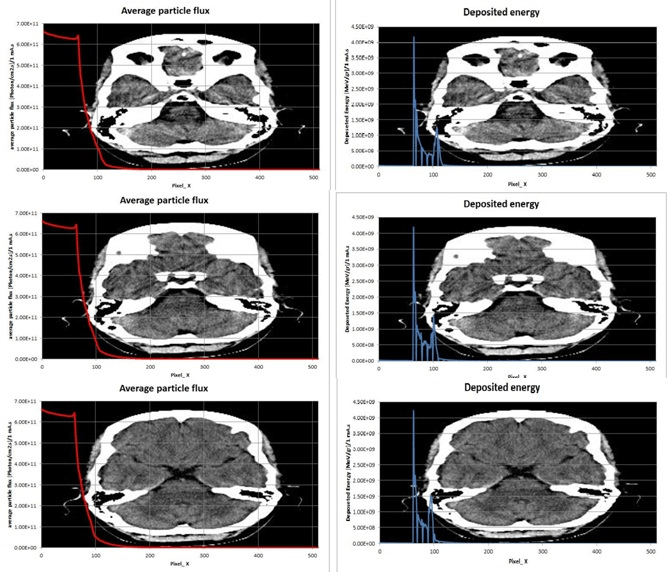
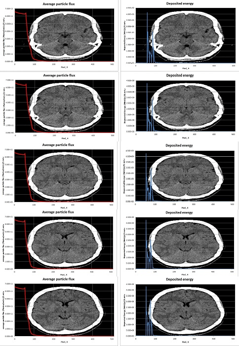
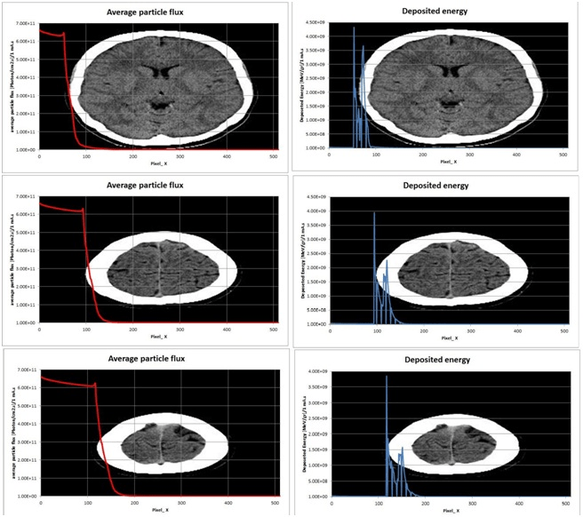
The number of radiation pulses that enter and/or traverse a medium is governed by inverse square law, which states that the flux of radiation emitted from a point source is inversely proportional to r², at the beginning of tissues (pixel’s number 100) most of X ray photons will be absorbed in the skin and skeleton—cranium bone because the value of total attenuation coefficient generally increase as the Z of the medium increases. where photoelectric interactions are increased in high-Z materials especially for low-energy photons.

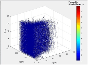
While Figure 6 shows the distribution of photons flux in the phantom, when the point source of X ray photons at z=10 cm (middle of scan length).

Figure 6. A Three-Dimensional Plot Representation of Photons Flux in the Phantom, When the Point Source of X ray Photons at z=10 cm (Middle of Scan Length)

DISCUSSION

In this research, we tried to use the available software to extrapolate and estimate the average particle flux, deposited energy, and mass attenuation coefficient depending on determine the mean free path of X-ray photons resulting at 120 kVp and 1 mAs as function to digital imaging and communications in medicine (DICOM) pixel numbers in the brain tissues for a 29-year-old female patient using MCNP code. Table 4 shows the change of deposited energy in (MeV/g /1mAs), mean free path (cm), and mass attenuation coefficient (cm²/g) as function to CT numbers of head CT images, these values can vary from one region to another according to CT numbers and their distribution and availability in each region, for example the abdominal region will contain the imaging numbers that represent the soft tissue at a higher rate than those representing the bones and cartilage. In this case (head scan images) the percentage of tissues with CT numbers less than 100 (except air between source and patient) equals to 87.11% and the sum of deposited energy over these regions equals to 1.77×10¹⁰ , but the tissues with CT numbers greater than 100 equals to 12.89% and absorbed dose in these tissues reach to 9.12×10⁹    . From Figure 5 X-ray photon flux can be reach to 6.30×10¹¹    at surface skin, this flux follows the inverse square law and drops to 10⁹   when passing the bones of the skull and skin where photons deposit most of their energy as shown in Figure 5.

The Comparison 

In order to validate the results obtained, these results were compared with a number of reference studies. Figure 7 shows a comparison between a plot of the energy spectrum of the X-ray photons calculated in this study at different voltage values and using an aluminum filter with thickness (1.2 mm) and a tungsten rotating anode with angle of 12°, with those of the reference.⁷

Figure 7. A comparison between a Plot of the Energy Spectrum of the X-ray Photons Calculated in This Study

Also, the effective dose calculated in this study was compared to the head region with those in the reference.⁸ The Table 5 shows the result of the comparison. Taking into account the weighting factor for tissue of the brain is 0.01 [ICRP 2007] and for bone and cartilage tissues is 0.01.

CONCLUSION

The DICOM images of brain were read and the intensity values were extracted and organized within 7864320×4 double matrix in order to build a three dimensional model for MCNP code input file in purpose to study of absorbed dose in the brain tissues for a 29-year-old female patient during CT scan of the head at specific voltage and current of X-ray tube using MCNP code and Matlab program. The Matlab program was used to read the DICOM images and extract the intensity values in each pixel of the image corresponding to certain slice of the brain. These color levels are characteristic of different tissue, and have been relied upon to create the specific material in each volume element in MCNP input file. As a result the absorbed dose in soft tissues with CT numbers less than 98 (which the percentage is 87.11%) can be reach to 0.222 Gy/1mAs, and for tissues with CT numbers greater than 98 (which the percentage is 12.89%) can be reach to 0.174 Gy/1mAs. These values for the dose are high, so it is always necessary to be cautious when performing the examination to obtain acceptable images from the first time and without having to repeat the imaging again for the same case unless there are necessities for it.

1. Kharita MH, Wali Kh Patient management practice in computed tomography with special emphasis to pediatric patients. Web site osti. https://www.osti.gov/etdeweb/biblio/21499832. Accessed May 19, 2019.

2. The MathWorks. The Mathworks Website mathworks. http://www.mathworks.com. Accessed April 2, 2019.

3. Mckinney G. MCNP — A General Monte Carlo N-particle Transport Code, Version 5. X-5 Monte Carlo Team. LA, USA: Los Alamos National Laboratory; 2003: 484.

4. Schneider U, Pedron E, Lomax A. The calibration of CT Hounsfield units for radiotherapy treatment planning. Physics in Medicine and Biology. 1996; 41(1): 111-124. doi: 10.1088/0031-9155/41/1/009

5. Massicano F, Massicano AVF, da Silv NG, Cintra FB, de Carvalho RM, Yoriyaz H. Analysis of CT and PET/SPECT images for dosimetry calculaion. Paper presented at: International Nuclear Atlantic Conference; 2009; São Paulo, SP – Brazil.

6. ASTAR and PSTAR databases. Web site physics.nist. https://physics.nist.gov/cgi-bin/Star/compos.pl?matno=201. Accessed May 19, 2019.

7. M R Ay 1, S Sarkar, M Shahriari, D Sardari, H Zaidi. Assessment of different computational models for generation of X-ray spectra in diagnostic radiology and mammography. Med Phys. 2005; 32(6): 1660-1675. doi: 10.1118/1.1906126

8. Radiological Society of North America (RSNA). Radiation Dose in X-Ray and CT Exams. Web site radiologyinfo. http://www.radiologyinfo.org. Accessed May 25, 2019.