INTRODUCTION
The basilar portion of the occipital bone and the occipital condyles are osteological elements frequently encountered by anthropologists in the field. Their relatively thick structures allow them to survive even in cases of poor preservation.1,2,3,4 Therefore, methods for identification of demographic variables employing this region of the skeleton would be particularly useful.
Research has been carried out on the occipital condyles of adults in attempts to create sex5,6,7,8,9 and biological affinity10 based methods for use in analysis of unknown individuals. The condyles have also been used with three dimensional (3D) imaging in association with the first cervical vertebra to aid in individuation in commingled situations.11
Research focusing on estimation of sex has been based on the ranges of sizes between males and females in the occipital, measured with hand held calipers12,13,14 and radiological images15,16 to calculate size and area; both of which are considered to be consistent data collection.16 Depending on geographic region the foramen magnum was included17 in some and excluded16,18 in other discriminant function analyses based on the “complete” crania to estimate sex. These models also require that geographic population is known prior to estimation of sex for an unidentified individual. Few specifically included measurements of the occipital condyles in their models.7,9,15
Traditionally researchers estimate age for non-adult skeletal remains based on the eruption19,20,21,22 or calcification,23,24,25,26 of the dentition.27 In cases where teeth are absent, epiphyseal fusion and long bone lengths can be used to estimate age.28,29,30 Many archaeological and forensic contexts include fragmentary and comingled skeletal remains, precluding the application of these traditional methods. In situations where traditional methods cannot be employed, alternative methods are needed to assess age in non-adults. In fact, Rissech et al31 state some authors have recently highlighted the need to increase and diversify the number of growth models based on direct measurements from documented osteological material, to elaborate reference data concerning the development of each skeletal element and to deepen our understanding of the development of the different populations.31p. 202
Research on the basicranium of non-adults has been studied as a potential way to estimate age for unknown individuals.3,32,33,34 It has been observed that just following birth the size of the pars lateralis increases significantly, with complete fusion of the four parts (pars lateralis, pars basilaris, squama) between 6-8-years of age, therefore by 6-8-years of age the area around the foramen magnum is close to the final adult size.3,9 A few of the studies have used archaeological samples observing the dentition or long bones to estimate age for comparison with occipital aging models.33,34 Many of these previously observed studies were individuals under 8-years of age3 and all were affected by small total sample sizes and for each year of life. As with studies conducted for sexing of adults, few of the studies of non-adults have included the occipital condyles specifically although there are a few exceptions.13,14,35,36 Standerwick et al35 observed that there is a measurable change with age in the length of the angle of the anterior aspect of the condyles but do not present a method for age estimation.
Redfield’s4 early research found metric change in the basicranium of non-adults that appeared stable across several samples, although sample sizes were small. Further, Redfield4 discussed the presence of morphological change occurring on the condyles calling them “condylar fossae”. The fossae do not occur where the condyles fuse together but at the canalis hypoglossi.31,p. 208 He states that the “condylar fossae” appear with the beginning of fusion between the pars lateralis and pars basilaris, and that in most individuals over the age of 12 this area has become smooth. Although it was also noted that occasionally an adult might have a persistent fossae in this location. Furthermore, authors agree that genetic disorders4 or resource deprivation do not affect growth and development of the basicranium.37,38 Use of the basicranium could be used in most cases where non-adults required aging.
Redfield’s4 research described the development of the occipital for specific age ranges to use in archaeological and forensic applications. However, it was developed using a skeletal sample where the age at death was unknown. The goal of the current study was to develop a system for aging similar to Redfield4 with specific focus on the occipital condyles.
Observations of the occipital condyles by the authors during previous research suggested that a process of morphological change was occurring during the course of development. The condyles of non-adults display billowing, depressions, grooves, and an even surface, changes that are similar to those observed on the bones of the auricular surface,39 pubic symphysis,40,41,42 and sternal rib ends.43,44 A similar pattern is observed during growth and development of billowing in non-adults and flattening with advancing. Thus, it was hypothesized that a relationship existed between the morphological features observed on the occipital condyles and age.
Another goal of the present study was to establish definitions for occipital condyle measurements developed specifically for unfused non-adults and fused adult/non-adult skeletal elements.
Previous research suggests that both metric and morphological change can be used to estimate differences in age based on the basicranium. The current research expands upon these earlier studies.
METHODS
The data collection procedure was two-fold, including both morphological and metric analyses. Two types of measurements, length (left occipital condyle length (LOCL)/right occipital condyle length (ROCL)) and width (left occipital condyle width (LOCW)/right occipital condyle width (ROCW)), were used to estimate the relationship between the size of the occipital condyles and age. Measurement descriptions for length and width of fused and unfused occipital condyles are as follows:
Adult/Fused Condyles
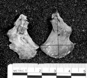
Maximum length of the occipital condyle-anterior to posterior margins of articular surface of the occipital condyle in the sagittal plane (Figure 1).
Figure 1. Fused (left) and Partially Fused (right) Measurements of Occipital Condyle Length/Width (A=Length, B=Width)
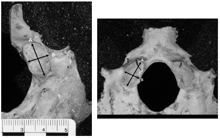
Maximum width of the occipital condyle-greatest width of the condyle perpendicular to length (Figure 1).
Non-adult/Unfused Condyles
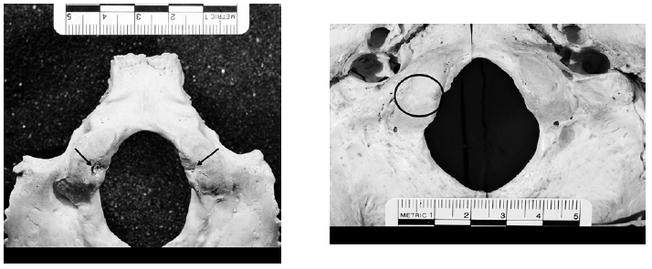
Maximum length of the occipital condyle-anterior to posterior margins of articular surface of the occipital condyle portion of pars lateralis in the sagittal plane (Figure 2).
Figure 2. Unfused Non-Adult Measurements of Occipital Condyle Length/Width (A=Length, B=Width)
Maximum width of the occipital condyle-greatest width of the condyle on pars lateralis perpendicular to length (Figure 2).
When taking the width measurements, if a natural groove transected the margin medially, the medial measurement was taken from the articular edge (groove is not included; Figure 3). All measurements were carried out with digital Mitutoyo calipers to the nearest 0.05 mm. Measurements were collected when possible on the left and right sides of the occipital condyles to test for variance. The ability to use either condyle alone may be needed in forensic and bioarchaeological cases.
Figure 3. Depression Breaking Margin (black arrows) and Bifurcated Condyle (circled in black)
The morphological analysis sought to develop descriptive features of the condyles based on changes in shape. This was performed via gross visual observation of the condyles, described as follows,
Billowing-low, rolling, medio-laterally positioned bumps (Figure 4).
Figure 4. Occipital Condyles Showing a (A) Depression, Groove (B), and Billow (C)
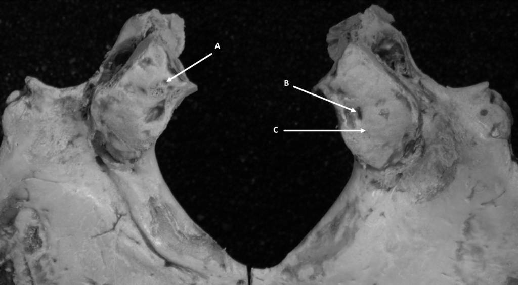
Depression-low relief circular, oval, and star shapes (Figure 4), enclosed on all sides; any depression crossing the medial margin does not fit this category and is a normal variation seen in adults and non-adults;
Grooves-low relief linear depression (Figure 4), enclosed on all sides; any groove crossing the medial margin does not fit this category and is a normal variation seen in adults and non-adults. Also excluded are the anterior suture lines on unfused condyles.
Nomenclature shown above describing the occipital condyles was purposefully similar to that used in describing the auricular surface39 and pubic symphysis40,41,42 to simplify the descriptive terms across methods of visual observation i.e. billowing.
These morphological features were recorded as present or absent and stage of fusion was observed as absent, partial, and completed.
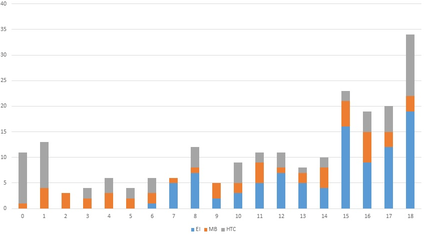
Condyles from three skeletal collections with known demographic information were assessed in this study. The hamann-todd collection (HTC) housed at the Cleveland Museum of Natural History provided 69 non-adults who died between 1912 and 1938.45 The Colecção Esqueletos Identificados housed at the Laboratory of Forensic Anthropology of the Life Sciences Department at the University of Coimbra Portugal, was made up of individuals that died between 1915 and 1942,46 providing 113 non-adults for observation. The Museu Bocage (MB) in Lisbon (National Museum of Natural History) provided 60 non-adults for observation, who died between 1880 and 1984.32,47 The skeletal remains from these three collections have thorough documentation making them excellent samples to use in the creation of the method outlined in this current research. Individuals ranging from fetal age to 18-years of age were observed. This resulted in a total of 242 individuals used in the morphological portion and 224 individuals formed the metric portion of the analysis as shown in Figure 5. Sex was recorded along with age, biological affinity and stage of fusion from the files accompanying the remains to assess variability for the HTC individuals only. While Redfield4 suggested pathological change in the basicranium did not affect growth and development individuals included in the current study were observed for presence or absence of pathology in the current study for consistency.
Figure 5. Number of Individuals by Age Category and Sample
The canonical discriminant analysis (a dimension-reduction technique related to principal components and canonical correlation) procedure in SAS 9.4 was used to obtain a set of linear combinations of the quantitative variables (ROCL, ROCW, LOCL and LOCW). These best reveal the differences among age (classification variable), sex (female/male), and stage of fusion (fused/unfused).
The approximate F-test tests the hypothesis that the given canonical correlation and all smaller ones are equal to zero in the population. The first tests if either dimension is significant and the second tests if dimension 2 by itself is significant. Larger values for the F statistic show better correlation, and can have similar significance to p-values of 0.0001.
Linear regression with backward selection was also carried out using SAS 9.4 to create age estimation formulae to be used by location and variable. The R2 produced by linear regression represents the percent of variance between the dependent variable and the independent variable. Values for R2 range from 0 to 1, with larger values suggesting increased linear correlation.
Intraobserver error measurements were taken on the HTC sample by the first author four weeks apart on a randomized sample of 12 individuals. The second author observed a randomized sample of 22 individuals from the HTC population four weeks following the first author’s original measurements to assess interobserver error. The absolute technical error of measurement (TEM) and relative technical error of measurement (rTEM) were calculated to test measurement precision for intra- and interobserver error, as they are broadly applied for measuring precision.6,48 rTEM offers a percentage of error while TEM shows the error in the same units as the original measurements; TEM values can be used as a form of standard deviation between repeated measurements.49 The coefficient of reliability (R) was also calculated for intra- and interobserver error, with an output range between 0 and 1. Values closer to 1 show excellent reliability for each measure.48
Regarding morphology, intraobserver error was observed for the HTC sample by the first author on a randomized sample of 11 individuals, while the second author observed a randomized sample of 20 individuals from the same HTC sample. McNemar’s test was used to explain the error for intra- and interobserver error for morphology change.
RESULTS AND DISCUSSION
Metrics
No pathologies on the basicranium were identified during observation of the three samples. Table 1 displays descriptive statistics for the three collections separately and the three pooled together. Results of summary dimension reduction for canonical discriminant analyses illustrating a set of linear combinations of the quantitative variables (ROCL, ROCW, LOCL and LOCW) that best reveal the differences among age using each of the three samples as well as the combined data are summarized in Table 2. Additional variables are also noted in Table 2 for the HTC including sex (female/male), biological affinity (black/white), and state of fusion (fused/unfused). A summary data reduction dimensions and canonical correlation analysis are shown in Table 3.
| Table 1. General Descriptive Statistics for all Cities, HTC, EI and MB Measurements |
| Variable |
N |
Mean |
Standard Deviation |
Coefficient of Variation |
Minimum |
Lower
Quartile |
Median |
Quartile |
Maximum |
| All Cities |
| ROCL |
230 |
21.49 |
4.34 |
20.18 |
6.95 |
19.81 |
22.63 |
24.23 |
27.8 |
| ROCW |
226 |
9.67 |
2 |
20.73 |
1.16 |
8.55 |
9.79 |
10.74 |
19.5 |
| LOCL |
225 |
21.41 |
4.37 |
20.41 |
6.51 |
19.99 |
22.36 |
24.22 |
28.6 |
| LOCW |
223 |
10.05 |
1.96 |
19.47 |
3.47 |
8.96 |
10.18 |
11.08 |
21.2 |
| HTC |
| ROCL |
68 |
19.24 |
5.52 |
28.72 |
6.95 |
14.59 |
21.3 |
23.4 |
26.8 |
| ROCW |
67 |
8.71 |
2.19 |
25.12 |
1.16 |
7.86 |
9.24 |
9.97 |
12.6 |
| LOCL |
65 |
19.09 |
5.61 |
29.37 |
6.51 |
14.92 |
21.14 |
23.39 |
27.3 |
| LOCW |
65 |
9.6 |
2.71 |
28.26 |
3.47 |
8.3 |
9.9 |
10.97 |
21.2 |
| EI |
| ROCL |
102 |
23.17 |
2.34 |
10.08 |
16.6 |
21.77 |
23.46 |
24.64 |
27.8 |
| ROCW |
101 |
10.42 |
1.77 |
16.95 |
6.55 |
9.37 |
10.2 |
11.34 |
19.5 |
| LOCL |
103 |
22.92 |
2.88 |
12.56 |
13 |
20.9 |
22.91 |
24.96 |
28.6 |
| LOCW |
99 |
10.61 |
1.44 |
13.53 |
6.87 |
9.58 |
10.62 |
11.4 |
14.5 |
| MB |
| ROCL |
60 |
21.19 |
4.26 |
20.11 |
10.2 |
18.33 |
22.23 |
24.14 |
27.4 |
| ROCW |
58 |
9.47 |
1.65 |
17.42 |
5.44 |
8.17 |
9.69 |
10.58 |
14.5 |
| LOCL |
57 |
21.34 |
3.87 |
18.15 |
10.6 |
19.86 |
22.26 |
23.43 |
27.6 |
| LOCW |
59 |
9.61 |
1.45 |
15.04 |
6.11 |
8.48 |
9.83 |
10.52 |
14.1 |
| HTC: Hamann-todd collection; EI: Elimination; MB: Museu bocage; ROCL: Right occipital condyle length; ROCW: Right occipital condyle width; LOCL: Left occipital condyle length; LOCW: Left occipital condyle width. |
| Table 2. Canonical Discriminant Analyses for All Cities, HTC/MB, EI, MB, and HTC |
| City |
Variable |
Dimension for RV vs LV |
Dimension for RV vs LV and G |
Dimension for RV vs LV and E |
Dimension RV vs LV and F |
| HTC/El/MB |
Right Variables |
1 |
2 |
1 |
2 |
1 |
2 |
1 |
2 |
| ROCL |
0.17 |
-0.19 |
|
|
|
|
|
|
| ROCW |
0.05 |
0.53 |
|
|
|
|
|
|
| Left Variables and Demographics |
|
|
|
|
|
|
|
|
| LOCL |
0.17 |
-0.26 |
|
|
|
|
|
|
| LOCW |
0.06 |
0.88 |
|
|
|
|
|
|
| HTC/MB |
Right Variables |
|
|
|
|
|
|
|
|
| ROCL |
0.18 |
-0.21 |
|
|
|
|
|
|
| ROCW |
0.08 |
0.67 |
|
|
|
|
|
|
| Left Variables and Demographics |
|
|
|
|
|
|
|
|
| LOCL |
0.18 |
-0.30 |
|
|
|
|
|
|
| LOCW |
0.09 |
0.86 |
|
|
|
|
|
|
| El |
Right Variables |
|
|
|
|
|
|
|
|
| ROCL |
0.56 |
-0.34 |
|
|
|
|
|
|
| ROCW |
0.14 |
0.32 |
|
|
|
|
|
|
| Left Variables and Demographics |
|
|
|
|
|
|
|
|
| LOCL |
0.48 |
-0.21 |
|
|
|
|
|
|
| LOCW |
0.24 |
1.18 |
|
|
|
|
|
|
| MB |
Right Variables |
|
|
|
|
|
|
|
|
| ROCL |
0.22 |
-0.17 |
|
|
|
|
|
|
| ROCW |
0.03 |
0.92 |
|
|
|
|
|
|
| Left Variables and Demographics |
|
|
|
|
|
|
|
|
| LOCL |
0.22 |
-0.25 |
|
|
|
|
|
|
| LOCW |
0.09 |
1.10 |
|
|
|
|
|
|
| HTC |
Right Variables |
|
|
|
|
|
|
|
|
| ROCL |
0.17 |
-0.21 |
0.18 |
-0.21 |
0.17 |
-0.21 |
0.18 |
-0.21 |
| ROCW |
0.08 |
0.61 |
0.07 |
0.61 |
0.08 |
0.61 |
0.07 |
0.61 |
| Left Variables and Demographics |
|
|
|
|
|
|
|
|
| LOCL |
0.16 |
-0.32 |
0.16 |
-0.14 |
0.16 |
-0.27 |
0.15 |
-0.08 |
| LOCW |
0.10 |
0.82 |
0.09 |
0.54 |
0.10 |
0.44 |
0.09 |
0.60 |
| Gender |
|
|
0.09 |
-1.80 |
|
|
|
|
| Bio. Affin. |
|
|
|
|
-0.06 |
1.97 |
|
|
| Fused |
|
|
|
|
|
|
0.27 |
-2.11 |
| Table 3. Data Reduction Dimensions and Canonical Correlation Analysis |
| City |
Dimension |
Canonical Correlation |
Adjusted Canonical Correlation |
Coefficient of Variation |
Approximate Standard Error |
Squared Canonical Correlation |
Eigenvalue |
Proportion |
F, Num df, Den df,
p-value
|
| Cleveland
Bio. Affin. |
1 |
0.95201 |
0.94855 |
0.017102 |
0.90633 |
9.6757 |
0.9903 |
20.96, 6, 52, <0.0001 |
27.8 |
| Cleveland
Bio. Affin. |
2 |
0.29445 |
0.24827 |
0.166744 |
0.08670 |
0.0949 |
0.0097 |
1.28, 2, 27, 0.2939 |
19.5 |
| Cleveland
Fused |
1 |
0.95544 |
0.95223 |
0.015909 |
0.91286 |
10.4762 |
0.9884 |
22.45, 6, 52, <0.0001 |
28.6 |
| Cleveland
Fused |
2 |
0.33136 |
0.29257 |
0.162527 |
0.10980 |
0.1233 |
0.0116 |
1.67, 2, 27, 0.2080 |
21.2 |
| Cleveland
Sex |
1 |
0.95265 |
0.94919 |
0.016881 |
0.90754 |
9.8154 |
0.9796 |
22.62, 6, 52, <0.0001 |
26.8 |
| Cleveland
Sex |
2 |
0.41223 |
0.38580 |
0.151549 |
0.16994 |
0.2047 |
0.0204 |
2.76, 2, 27, 0.0809 |
12.6 |
| Cleveland
No Demographics |
1 |
0.95187 |
0.95006 |
0.017150 |
0.90606 |
9.6457 |
0.9941 |
31.79, 4, 54, <0.0001 |
27.3 |
| Cleveland
No Demographics |
2 |
0.23260 |
. |
0.172697 |
0.05410 |
0.0572 |
0.0059 |
1.60, 1, 28, 0.2161 |
21.2 |
| Cleveland-
Coimbra-
Lisbon |
1 |
0.97037 |
0.96981 |
0.007732 |
0.94163 |
16.1309 |
0.9978 |
86.71, 4, 108, <0.0001 |
27.8 |
| Cleveland-
Coimbra-
Lisbon |
2 |
0.18497 |
. |
0.127921 |
0.03421 |
0.0354 |
0.0022 |
1.95, 1, 55, 0.1684 |
19.5 |
| Cleveland-
Lisbon |
1 |
0.95961 |
0.95858 |
0.011931 |
0.92086 |
11.6356 |
0.9905 |
56.34, 4, 82, <0.0001 |
28.6 |
| Cleveland-
Lisbon |
2 |
0.31742 |
. |
0.135566 |
0.10076 |
0.1120 |
0.0095 |
4.71, 1, 42, 0.0358 |
14.5 |
| Coimbra |
1 |
0.91649 |
0.90794 |
0.046200 |
0.83996 |
5.2483 |
0.9926 |
6.97, 4, 18, 0.0014 |
27.6 |
| Coimbra |
2 |
0.19360 |
. |
0.277856 |
0.03748 |
0.0389 |
0.0074 |
0.39, 1, 10, 0.5466 |
14.1 |
| Lisbon |
1 |
0.98607 |
0.98494 |
0.007674 |
0.97233 |
35.1428 |
0.9926 |
28.77, 4, 20, <0.0001 |
14.1 |
| Lisbon |
2 |
0.45587 |
. |
0.219711 |
0.20782 |
0.2623 |
0.0074 |
2.89, 1, 11, 0.1174 |
14.1 |
The current research shows that dimensions 1 and 2 are each significant for side, sex, biological affinity, and fusion. Since the p-value is equal to <0.0001, less than the standard 0.05 indicator of significance it was concluded that the canonical correlations are not zero and therefore represent linear relationships within each of the variables.
The approximate F-test tests the hypothesis that the given canonical correlation and all smaller ones are equal to zero in the population. The first tests if either dimension is significant (F=145.95, 4, 408, <0.0001). The second tests if dimension 2 by itself is significant (F=29.55, 1, 205, <0.0001). Therefore, dimensions 1 and 2 are both significant. Since p≤0.0001 is less than 0.05 we can conclude that the canonical correlations are not zero and there is a linear relationship between the two groups of variables.
The squared canonical correlation for 1 and 2 combined is 0.806368. That is, approximately 80.6% of the variation in set 1 is explained by set 2, or vice versa. Hence, one could employ either set one (left) measurements or set two (right) measurements. It appears that age distribution drastically affects the squared canonical correlation for 1 and 2 combined. Note for Coimbra the squared canonical correlation is about 34%.
For HTC biological affinity, sex, and fusion the first canonical correlation coefficients are above 0.95 with an explained variance of the correlation above 98%, eigenvalues of 10-11.2973, and p<0.0001.
A one unit increase in ROCL leads to a 0.21 unit increase in the first variate of the Right measurements (“Right1”), when ROCW is held constant and a one unit increase in LOCL leads to a 0.20 unit increase in the first variate of the Left measurements (“Left1”), when LOCW is held constant.
The first canonical correlation coefficient for HTC (without demographics) and Lisbon are over 0.91, with explained variance of correlation of 96-98%. All Cities almost reach 90% for the first canonical correlation coefficient at 0.897980 with an explained variance of the correlation of 96.65%, and a p<0.0001.
Coimbra provided a much different first canonical correlation coefficient of 0.582923, with an explained variance of the correlation of 77.47%, and a p<0.0001.
Using only Lisbon and Cleveland combined the R2 is 58%. Including Coimbra in the All Cities sample increases the overall categorical size but decreases the R2 considerably.
The adjusted R2 for the linear combination of the measured variables (LOCW, LOCL, ROCW, ROCL) and age using backward elimination are 0.70, 0.33, and 0.43 for HTC, MB and All Cities combined respectively (Table 4). All variables were removed using backward elimination (EI) leaving the intercept only. The following are equations meant to produce estimated age using linear regression with backward selection:
All Cities: Predicting age using left and right measurements
Age=-10.05559+(0.42252*ROCL)+(0.33422*LOCL)+(0.60259*LOCW)
Coimbra: Predicting age using left and right measurements
None with statistical significance to create an equation for prediction.
Lisbon: Predicting age using left and right measurements
Age=-8.57785+(0.98134*LOCL)
Cleveland: Predicting age using left and right measurements
Age=-12.57180+(0.87680*ROCL)+(0.49794*LOCW)
Cleveland: Predicting age using left and right measurements and fused
Age=-8.15237+5.48057*Fused+0.50296*LOCL
Cleveland: Predicting age using left and right measurements and biological affinity
Age=-11.81444+-2.62040*Bio.Affinity+0.84622*LOCL+0.71060*LOCW
TEM for intraobserver error suggested that the most reliable measurement was LOCW and the variable with the least reliability was LOCL. TEM for interobserver error showed ROCW as the most reliable measurement, while LOCL was the variable most affected by human error. Intraobserver rTEM ranged from 0.89 for ROCL to 2.36 for LOCL. Interobserver rTEM ranged from 1.07 for ROCL to 2.18 for LOCW. R2s were over 0.99 for each of the four measurements using TEM for intra- and inter-observer error. This suggests 99% of error is due to a factor other than author measurement error.
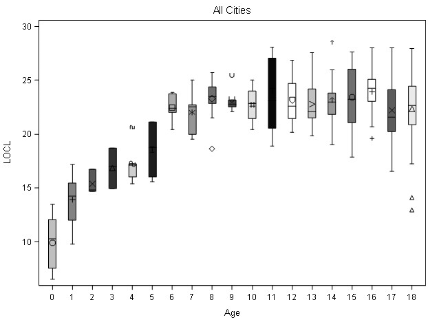
Box plots were prepared to observe if data lumping for all cities combined could be used as a strategy to create intervals for age estimation. Figure 6 illustrates the distribution of for each age group. The data indicate that size is not associated with a specific age (1-year of age) or specific age intervals (1-3-years of age). Instead the data suggest that the raw canonical coefficients should be interpreted in a manner analogous to interpreting regression coefficients i.e., for the variable age, a one unit increase leads to a 0.1449 increase in the first canonical variate when all of the other variables are held constant.
Figure 6. LOCL Box Plot for Samples Combined by Millimeters and Age
Morphology
The model was first applied to the HTC sample where four morphological factors were found to be associated with age, including stage of fusion, presence/absence of billowing, presence/absence of depressions, and presence/absence of grooves. Grooves that break the medial condylar margin and bifurcated condyles are not factors in aging (Figure 3). Fusion was present as early as 3-years of age and all non-adults over 8-years showed 100% complete fusion. If an individual’s condyles displayed fusion but still displayed grooves, billowing or depressions there was a 92% chance that they
would fit into the 3-13-year-old age range. Generally flattened condyles were observed after age 13; however, 53% of unfused non-adults under three years of age were also flat. These results do not offer a “morphological method” but provide observations of morphological features present during the growth and development period from 3-13-years of age. Of the 196 fused individuals in the combined sample, 16 did not fit the pattern of fusion and were under aged.
For the HTC, 31 females and 37 males were observed. One female and five males did not match the presence/absence expected for morphological features associated with age resulting in 10% of the population being aged incorrectly. Thirty-females and 30 males were observed for morphology from MB; of these there were one female and one male that did not present the morphological features associated with age. Thus, 6% of the individuals would have been misidentified in terms of age for the MB non-adults. At EI 55 females and 58 males were observed for morphology; eight males did not show the morphological features associated with age and thus these eight would have been assigned an incorrect age. Misidentification of age at EI was at 7%. Combined the three samples resulted in a total of 231 individuals, with 16 fused individuals misclassified, meaning 92% were given an accurate age using the presence/absence of the morphological features defined here.
McNemar’s test, applied to study intraobserver error resulted in one disagreement for the variable of presence/absence of 11 individuals observed. McNemar’s test statistic suggests that there is not a statistically significant difference in the proportions of features described as presence/absence (p>1.000). Application of McNemar’s test to analyze interobserver error showed no discordant pairs between the two observers.
The EI sample population did not include individuals under the age of 6-years for observation making comparisons to the other sample populations unsuitable. The squamous cell carcinoma (SCC) values from the HTC show that if sex, biological affinity, or state of fusion are known specific equations would create more accurate age estimates (Table 4).
| Table 4. Parameter Estimates and Fit Statistics Explaining AGE Linear Models |
| City |
Variable |
Estimate |
StdErr |
t Value |
Probt |
LowerCL |
UpperCL |
| Cleveland
(Bio. Affin.)
n=64,
Adj. R-Square=0.72,
RMSE=3.74 |
Intercept |
-11.81444 |
1.90241 |
-6.21 |
<.0001 |
-15.61983 |
-8.00905 |
| Bio. Affin.=Black |
-2.62040 |
1.21898 |
-2.15 |
0.0356 |
-5.05872 |
-0.18208 |
| LOCL |
0.84622 |
0.11064 |
7.65 |
<.0001 |
0.62491 |
1.06753 |
| LOCW |
0.71060 |
0.23903 |
2.97 |
0.0042 |
0.23247 |
1.18874 |
| Cleveland
(Fused)
n=64,
Adj. R-Square=0.74,
RMSE=3.59 |
Intercept |
-8.15237 |
2.24440 |
-3.63 |
0.0006 |
-12.64184 |
-3.66291 |
| Fused=Yes |
5.48057 |
1.72187 |
3.18 |
0.0023 |
2.03632 |
8.92481 |
| LOCL |
0.50296 |
0.15012 |
3.35 |
0.0014 |
0.20269 |
0.80324 |
| LOCW |
0.41729 |
0.22519 |
1.85 |
0.0688 |
-0.03316 |
0.86774 |
| Cleveland
(No Demographics)
n=65,
Adj. R-Square=0.70,
RMSE=3.81 |
Intercept |
-12.57180 |
1.91048 |
-6.58 |
<.0001 |
-16.39079 |
-8.75282 |
| ROCL |
0.87680 |
0.11730 |
7.48 |
<.0001 |
0.64232 |
1.11127 |
| LOCW |
0.49794 |
0.23671 |
2.10 |
0.0395 |
0.02477 |
0.97112 |
| Coimbra
n=105,
Adj. R-Square=0.00,
RMSE=3.60 |
Intercept |
13.83810 |
0.35086 |
39.44 |
<.0001 |
13.14234 |
14.53385 |
| Lisbon
n=56,
Adj. R-Square=0.33,
RMSE=5.30 |
Intercept |
-8.57785 |
4.10612 |
-2.09 |
0.0414 |
-16.81013 |
-0.34557 |
| LOCL |
0.98134 |
0.18847 |
5.21 |
<.0001 |
0.60349 |
1.35919 |
| Cleveland/Coimbra/Lisbon
n=211,
Adj. R-Square=0.43,
RMSE=4.43 |
Intercept |
-10.05559 |
1.81934 |
-5.53 |
<.0001 |
-13.64240 |
-6.46879 |
| ROCL |
0.42252 |
0.15518 |
2.72 |
0.0070 |
0.11659 |
0.72846 |
| LOCL |
0.33422 |
0.14528 |
2.30 |
0.0224 |
0.04780 |
0.62063 |
| LOCW |
0.60259 |
0.18485 |
3.26 |
0.0013 |
0.23816 |
0.96701 |
The following examples display application of equations from Table 4 to a 12-year-old female from the HTC collection.
HTC only
Age=-12.57180+(0.87680*ROCL)+(0.49794*LOCW)=
9.57 years+/-3.81
Age=-12.57180+(0.87680*24.62)+(0.49794*11.46)
All Cities Combined
Age=-10.05559+(0.42252*ROCL)+(0.33422*LOCL)+(0.60259*LOCW)=15.41+/-4.43
Age=-10.05559+(0.42252*24.62)+(0.33422*24.46)+ (0.60259*11.46)
The HTC equation under aged this 12-year-old individual by ~2.5-years and for the All Cities combined equation the individual was over aged by ~3.5-years. If the root mean error is applied this individual would be within the ages of 5.7569 and 13.3831-years for the HTC only equation with a range of error 7.6262-years and between the ages of 10.98292 and 19.83708 using the All Cities model with a range of error 8.85416-years. Dental eruption by comparison ranges from +/-2-months to +/-36-months, total range of 6-years possible.27 Using the humerus as an example, standard deviations of long bone lengths can vary from between 5.42-12.11-years of age.50 Using the humerus again to look at fusion an age range between 17-24-years (head, distal epiphysis, and medial epicondyle)28 is suggested.
All three samples overlap by death dates and are considered to represent individuals of low to middle socio-economic status.31,51,52,53 The fact that the method does not work in the Coimbra sample is likely due to the fact that there are no individuals under six years of age present. These ages in the developmental period normally show lack of fusion.
Although the two Portuguese samples are geographically close Inskip et al5 state that for sex “there is enough variation between the European groups…to significantly impact the accuracy of sex assessment discriminant functions”.15p. 681 Veroni et al13 used length and width of the occipital condyles to assess sex in non-adults with a 75.8% accuracy for individuals over 8-years of age.13p. 149-150 On the other hand, Cardoso et al47 make the point that methods for age estimation should be both pooled and by sex; both were calculated for the HTC. In cases where sex is unknown the pooled population is best and when sex is known there would be an increase in the accuracy of the age estimate. In this paper it is suggested that methods for estimating non-adult age from occipital condyle measurements may still require populationally specific models as the three sample populations used here are mostly comprised of individuals of Western European descent. Socioeconomic status is considered low in all three collections but variation may also be present due to other environmental factors.5 These environmental factors and human growth in general can be quite variable making some authors31,54,55 believe age estimation methods on samples such as these should be used with caution.
The majority of the remains in all three collections represent individuals that were deemed poorest of the poor and were not given the same burial treatment as those of higher socio-economic status.56 Furthermore, Rissech et al31 discussed the size differences in children from Portuguese and English samples from the recent historic period with modern children and found that modern children are larger adding to an increase in temporal disparity. However, Redfield4 states that the base of the developing skull is stable and less likely to be affected even by conditions distorting the superior crania. This suggests the basicranium may not vary as other areas of the skeleton based on socioeconomic status and temporality. To better understand the effects of socio-economic status a study would need to research a sample of individuals with high socio-economic status.
TEM and R2 all show excellent precision between measurement trials for the first author and between authors indicating the measurements would be useful in future studies of non-adult occipital condyles. rTEM was only under 1% for intraobserver ROCL showing this to be the most reliable measurement. Together these show the measurements themselves are easily replicated.
Each morphological variant was distinct; presence of features were unable to be linked to “phases” or particular age ranges as seen in sternal rib ends, the auricular surface of the ilium, or pubic symphysis. While variation definitely exists in the developing occipital condyles, none of the specific changes, including billowing, depressions, and grooves, follow definable age ranges. Sixteen of the 196 fused individuals observed for morphological features did not fit into the age range 3-13, making the model 92% accurate. These observed changes do not include the medial depression that crosses the condyle’s margin or lines associated with complete or partial bifurcation of the condyles. This suggests that most of the morphological features seen on the occipital condyles are present between the ages of 3-13, encompassing the time the condyles begin and complete the fusion process. The upper age limit of 12 suggested by Redfield4 for disappearance of the “condylar fossae” fit within the method described here.
CONCLUSION
Measurements of length and width did not prove to be reliable methods for predicting age of the occipital condyles. As seen in prior studies total sample sizes of individuals under 6-years of age were small, only 26 at HTC and 15 at MB, where the metric method was significant. There were also no individuals represented for certain ages in this study including 2-years of age, 7 and 9-years of age for the HTC sample. To build upon the research presented here, additional data collection using documented collections focusing on increasing sample sizes, especially in certain age groups, are needed to improve our understanding of the potential for metric methods on the occipital condyles. As Standerwick et al35 observed change in the angle of the condyles during growth and development this is another area open to research potentially using 3D digitizer models.
Presence of billowing, depressions, and grooves can be used as a quick age assessment for the occipital condyles of unknown individuals to be between 3-13-years of age. Only presence, and not absence of billowing, depressions, or grooving can be used to estimate age. While morphological changes do exist on the condyles of non-adults the variation does not progress through specific morphological variables (ex. 1) billowing 2) billowing with depressions) at an identifiable pace. The changing morphology seen on the occipital condyles can age individuals between 3-13-years with 92% accuracy. The morphological changes of the occipital condyles allow researchers to meet the 80% accuracy Daubert criteria needed for forensic cases.57 Application of the morphological method should be limited to populations from similar geographic locations, the US and Southern Europe, those from the historic period to present, and those likely of lower socio-economic status. The morphological method should also be used in combination with other aging methods when possible. Even when considering the limitations, the morphological method adds a new tool to use in the age estimation of non-adult individuals in forensic cases, especially those with fragmented remains.
INSTITUITIONAL REVIEW BOARD PERMISSION
Not needed.
CONFLICTS OF INTEREST
The authors declare that they have no conflicts of interest.